
Abstract
The strict mathematical relationship between Rt and the curve of daily cases f(t) is shown. Up-to-date and statistically robust Rt from the curve of daily cases can be estimated as soon as new cases are added to the curve. That is equivalent to estimating Rt by averaging all detected cases of infection, without any distortion induced by the difficulty of following and weighting trees of secondary cases from original ones, and without needing to wait for secondary cases to manifest infection. With this method, if Rt scaled numbers are of interest, only the average duration of infectivity of subjects has to be estimated directly, but independently of linking secondary cases to primary ones. A new index, instantaneous reproduction number Rist is introduced, which does not depend on the duration of infectivity of subjects. Rist, Rt and the doubling/halving time of the epidemics may be estimated by simple computations at the very detection time of new daily cases. Any smoothed curve of daily cases gives smooth Rt and Rist. No phase lag on Rt estimate is introduced by this method.
Motivation for the method described here
I am new to epidemiology. I began to think about Rt during the first outbreak of COVID19 epidemics in Italy, while I was tinkering with a diffusion-saturation model trying to fit epidemic data: http://adaptive.it/covid19/. So, I do not know if what I found is new, or trivial, or already perfectly know. Excuse me for that. I am submitting my findings to the community in hope they may help.
During the first phase of COVID19 epidemics I encountered estimations of Rt which where incompatible with the doubling time of daily cases and the location in time of the peaks. So, I began to think on the subject.
It seems that Rt was defined from the epidemiological point of view with the assumption in mind that an epidemics can be characterized by a somewhat stable relationship between a pathogen and its infectable host. This in the hope of predicting the evolution of an outbreak. Which is not.
In fact, the initial susceptibility of a population of hosts is always unknown because unknown is the reaction of the immune system spectrum and history of a population. Besides that, both pathogen and host can modify this relationship via several options (decreasing susceptibility of the host population due to the spreading of the epidemics that saturates a population or sub-population of susceptible individuals, reaction of immune systems, reactive behaviors of the host and the pathogen populations, etc).
This writing shows how Rt definition is strictly tied to the curve of daily cases by mathematical equations. The two are essentially the same thing expressed with different words. Rt is a sort of first derivative of the curve of daily cases with respect to time t.
The difficulty of directly estimating Rt in a reliable way is the same as predicting the evolution of an epidemics in a reliable way. Indeed even much harder, since one has to face the further uncertainty of estimating trees of secondary cases, with all the uncertainty implied by this process. It is very similar to estimating the space traveled by measuring acceleration with very inaccurate accelerometers, but very much harder and error prone.
The excellent articles by Cori, et al. [2] and Dietz [3] clearly show this difficulty.
Epidemiological definition of Rt
The epidemiological definition of Rt states:
Rt is the number of secondary infections caused by a single case of disease during its period of infectivity in a completely susceptible population, on average.
(see: https://en.wikipedia.org/wiki/Basic_reproduction_number [5])
According to this epidemiological definition, Rt is analogous to the multiplier of the initial unit capital after 1 period, in a compound capitalization process.
This analogy allows the estimation of Rt from the epidemic curve of daily cases by introducing the concept of Instantaneous Reproduction Number Rist, similar to the instantaneous capitalization rate in actuarial mathematics.
Definition of Rist
The epidemiological definition of Rt (and its cousin R0, as its limit to the beginning of an epidemics of an uninfected population) indicates an exponential expansion. An infected, after his period of infectious capacity will have infected a new infected plus (or minus) a number of new infected individuals. Let’s say, for example, one infected plus another one and a half infected, equal to two and a half infected (1 + 1.5 = 2.5). After 2 periods of infectivity, the infected will be those of the previous period (2.5) each of which will have infected new ones (1 + 1.5 = 2.5): i.e. the (1 + 1.5) of period 1, multiplied by (1 + 1.5) of period 2; and so on…
In general:
after period 1: 1 · (1 + r) = Rt;
after period 2: 1 · (1 + r) · (1 + r) = 1 · (1 + r)2;
and so on: (1 + r)1, (1 + r)2 … (1 + r)p.
In fact, this is a process equivalent to the amount of a compound capitalization of the interest rate r, where Rt is the amount after period 1.
To obtain which interest rate r should be used for a continuous compound capitalization of n fractions of a period that gives the amount Rt after 1 period, we can write as follows:
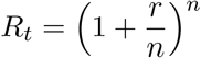 equivalent to
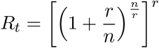 Passing to the limit for n → ∞, and noting that
 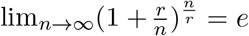 , we get:
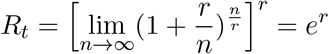 hence
hence
 In other terms, r is the exponent to be given to e to obtain Rt after a period of infectious duration equal to 1. That is:
 If we want to express Rist in a unit of time gi other than the dimensionless unit period, for example the days (or hours) with which we measure the duration of the infectivity period of an infectious subject and with which we measure the progress of the epidemic, we can write:
 from wich:
 In this way we have the parameter Rist which characterizes the exponential growth (as per the definition of Rt) at the point in time t that the increase (or decrease) of the daily cases generates.
Connecting Rist to the epidemic curve of daily cases
Whenever an exponential function y = eax is represented in logarithmic scale ln(y) = ax, it becomes a straight line. Its shape factor a becomes the slope of the straight line (the angular coefficient).
If we represent the curve of the daily cases f(t) in logarithmic scale h(t) = ln(f(t)), the slope of the tangent of h(t) at point t is the slope Rist, corresponding to the exponential growth of the epidemiological definition of the effective reproduction number Rt, represented in logarithmic scale, at time t, and scaled in time units of the curve of daily cases. But the tangent of h(t) at point t is also the first derivative of h(t)
that is:
 A different reasoning perhaps better illustrates the concept of estimating Rt from epidemic curves.
Rt is basically the ratio between the daily cases at time t + 1 compared to the cases at time t, where 1 is the infecting period. Given the point a on the curve of daily cases that precedes the point b, then Rt = b/a.
Differentiating the curve of daily cases, expressed in logarithmic scale with base e, means making the difference between two values, spaced by a unitary period of time tending to zero, that is: ln(b) − ln(a). This expression is equivalent to doing ln(b/a), as those who have used slide rules easily remember: ln(b) − ln(a) = ln(b/a). (see: https://en.wikipedia.org/wiki/Slide_rule)
By doing the inverse operation of extracting a logarithm from a number, i.e. raising the base of the logarithm to a power of the value of the logarithm in question, one obtains the ratio b/a in the scale of daily cases of infection: eln(b/a) = b/a.
This ratio represents the rate of increase (if > 1), or decrease (if < 1), of the infections averaged over all the infections observed, including all the information on the overall average resistance to the spread of the infection that may have formed meanwhile, for any known or unknown reason it was formed. It also takes in properly weighted account all the overlappings of the infection trees defined by Rt and of the varying susceptibility of the hosts.
Furthermore, the value obtained in this way is a very accurate value of Rt acting at current time of b, that is, at the very moment in which the current value of the infected cases is known. The passage to the limit of a period that tends to the instant, implicit in the differentiation operation with respect to t, allows to have a curve of Rt trend that is always updated in real-time.
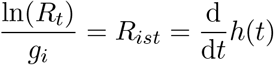
According to the epidemiological definition of Rt, we have the following correspondence of classical outstanding cases, direct consequence of that epidemiological definition:
Rist > 0
when the daily cases increase and the epidemic is expanding: therefore the associated 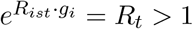 .
.
Rist = 0
when the daily cases remain constant and the epidemic is stationary:
therefore the associated 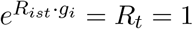 .
.
In this case the curve of daily cases has a minimum or a maximum;
Rist crosses 0; Rt crosses 1.
Rist < 0
when the daily cases decrease and the epidemic is contracting: therefore the associated 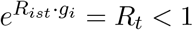 .
.
Since these outstanding cases derive from the epidemiological definition of Rt, they also are criterion for evaluating the correct estimate of Rt. A contrasting value of Rt respect to the epidemic curve is also an indication that Rt or the epidemic curve are wrong.
Summary of conversion formulas
The curve of daily cases f(t) expressed in logarithmic scale with base e is obviously given by:
 Rist is given by the first derivative (numerically or analytically determined) of any smoothed curve of daily cases, given in logarithmic scale with base e:
 Please notice that if we have a smoothing procedure of the curve of daily cases that introduces any phase lag, as we have using mobile averages or FIR/IIR filters, we will have the same phase lag in the estimation of Rist and Rt. Otherwise if we have some form of static averaging, as using some least squares fitting procedure, no phase lag is introduced.
Rt is given by:
 Rist is also equivalen to:
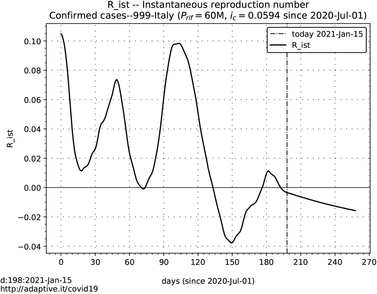
 The doubling or halving time of infection gd∨h is given by imposing 2.0 as Rt and computing the number of resulting days (negative numbers represent halving time):
Some charting outcome
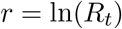
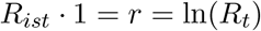
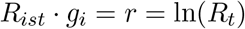
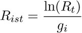
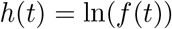
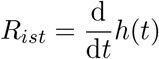
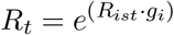
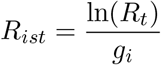
The following charts show how Rt may be estimated starting from a fitting of the curve of cumulative cases, with a sort of derivative of order 2. The curve of daily cases obviously is the first derivative of cumulative cases.
The fitting is primarily done on cumulative cases because they automatically compensate some kind of errors (for example: a missed case one day may be detected in the following days, etc.). Model and fitting techniques used for the following figures are outside the scope of this writing. Here the model is simply used as source of a smoothed daily data set. The other formulas used to generate the following charts are summarized in the section above. The datasource used for this fitting is the COVID-19 official one for Italy: https://github.com/pcm-dpc/COVID-19/ [1]
Just a glance at the dispersion of a ample set of daily data around a good fitting of these data let easily imagine how difficult and unreliable could be any attempt to estimate a trend of the epidemics from small samples of their derivatives and relying on considerations of the spread of these samples over overlapping trees of secondary cases, which is what the epidemiological definition of Rt asks to do.
Moreover, the dynamics of an epidemic seems to follow unpredictable and chaotic behavior. We are used to think of populations involved in an epidemic as an isotropic material, like steel, which has equal behavior in all directions respect to stress and strain.
Perhaps, an epidemics may be better depicted as acting on many different relationship fabrics entangled together. A burst of infections occurs when two or more entangled fabrics – which may be in a stable infective condition that eventually saturate – mix and new connections merge in a new more extended fabric.
If this is a plausible landscape of an infection of a population, not every link in this entaglement of networks has the same infection capacity and not all nodes of these networks are isotropically connected.
In other words there may be several networks that may have poor connections with each other, while having strong connection among the members of each network. For example, the network of families with children that go to the same school may have strong link between families of teachers and classmates, but may have weak connections with other unrelated networks of parentschildren-teachers. Some of these networks may saturate eventually, while others may not have even been infected. The same thing happens with other types of relational networks. This is a very anisotropic environment.
This landscape shows a very challenging non linear object to investigate. Maybe it has some emerging regularities at the macroscopic level, like sequences of overlapping sigmoidal shapes in the curve of cumulative cases.

Data fit with an adaptive diffusion/saturation model on cumulative cases. Model and fitting techniques used for these charts are outside the scope of this writing. Fitting model and details at http://adaptive.it/covid19/ [4] data-source:https://github.com/pcm-dpc/COVID-19/ [1]

Daily cases smoothed by fitting, in logarithmic scale with base e. Fitting model and details athttp://adaptive.it/covid19/ [4] data-source:https://github.com/pcm-dpc/COVID-19/ [1]

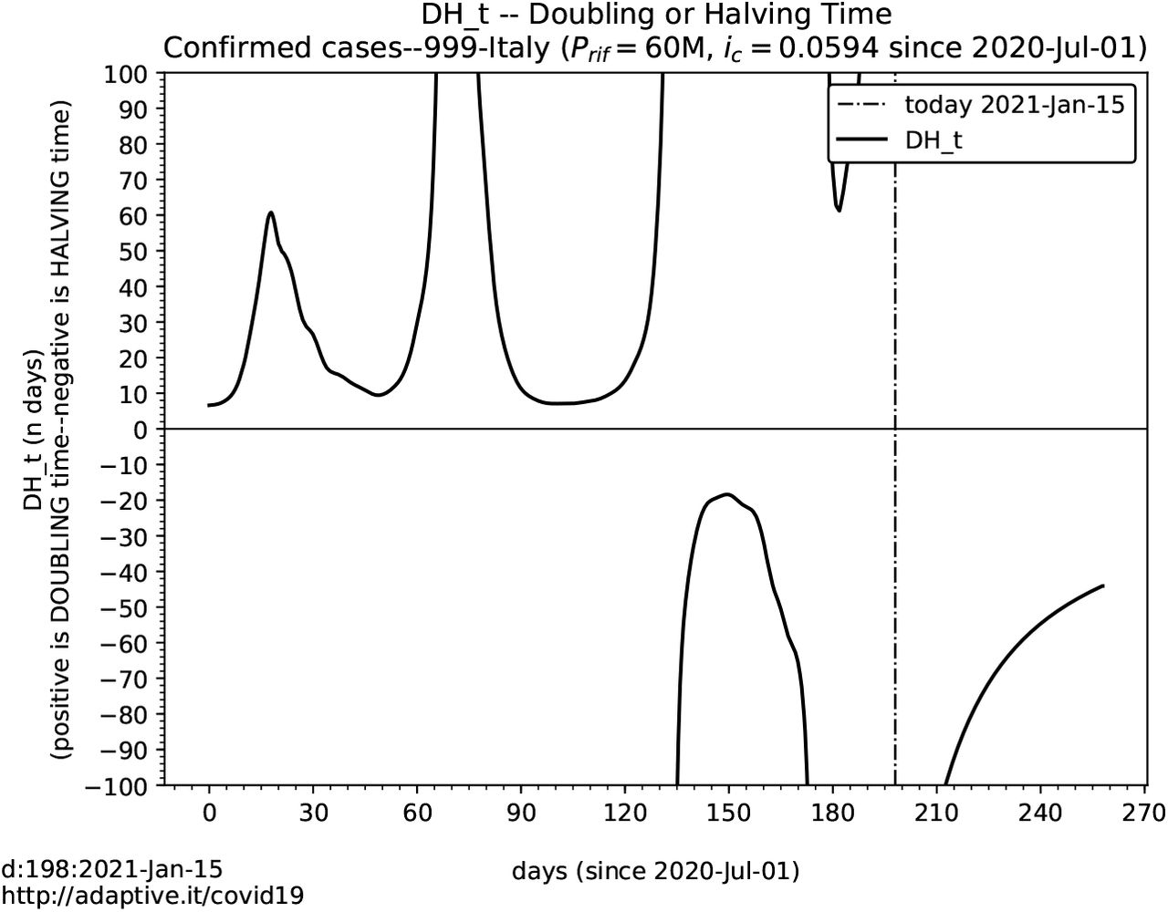
Computed Rt from smoothed daily cases in logarithmic scale with base e. Fitting model and details at http://adaptive.it/covid19/http://adaptive.it/covid19/ [4] data-source:https://github.com/pcm-dpc/COVID-19/ [1]
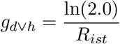
Computed Rist. Fitting model and details at http://adaptive.it/covid19/ [4] data-source:https://github.com/pcm-dpc/COVID-19/ [1]
Computed doubling/halving time (days). Negative values mean halving time. Fitting model and details at http://adaptive.it/covid19/ [4] data-source:https://github.com/pcm-dpc/COVID-19/ [1]
Data Availability
All the data used are of public domain. The mathematical model used is made by the author.


