
Abstract
The article is devoted the parameters identification in the SI model. We consider several method, starting from Liu et al. [17] to fit the early cumulative data of Sars-CoV2 in mainland China. This method provides a way to compute the parameters at the early stage of the epidemic. Next, we establish an identifiability result in the spirit of Hadeler [19]. Then we use the Bernoulli-Verhulst model as a phenomenological model to fit the data and derive some result on the parameters identification. The last part of the paper is devoted to some numerical Algorithms to fit a daily piecewise constant rate of transmission.
1 Introduction
Estimating the average transmission rate is one of the most crucial challenges in the epidemiology of communicable diseases. This rate conditions the entry into the epidemic phase of the disease and its return to the extinction phase, if it has diminished sufficiently. It is the combination of three factors, one, the coefficient of virulence, linked to the infectious agent (in the case of infectious transmissible diseases), the other, the coefficient of susceptibility, linked to the host (all summarized into the probability of transmission), and also, the number of contact per unit of time between individuals (see Magal and Ruan [1]). The coefficient of virulence generally decreases over the course of the disease history, due to favorable mutations (favorable to the host). The second and third also, if mitigation measures have been taken. This was the case in China from the start of the pandemic (see Qiu, Chen and Shi [2])). Monitoring the decrease in the average transmission rate is an excellent way to monitor the effectiveness of these mitigation measures. Estimating the rate is therefore a central problem in the fight against epidemics.
The goal of this article is to understand how to compare the SI model to the reported epidemic data and therefore can be used to predict the future evolution of epidemic spread and to test various possible scenarios of social mitigation measures. For t ≥ t0, the SI model is the following
 where S(t) is the number of susceptible and I(t) the number of infectious at time t. This system is supplemented by initial data
 In this model, the rate of transmission τ (t) combines the number of contacts per unit of time and the probability of transmission. The flux of new infectious is described by a mass action law τ (t) S(t) I(t).
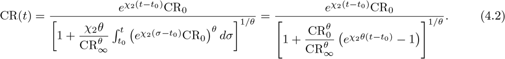
The quantity 1/ν is the average duration of the infectious period and νI(t) is the flux of recovering or dying individuals. At the end of the infectious period, we assume that a fraction f ∈ (0, 1] of the infectious individuals is reported. Let CR(t) be the cumulative number of reported cases. We assume that
 Where
Where

We assume that
S0 > 0 the number of susceptible individuals at time t0 where we start to use the model;
 the average duration of infectious period;
f > 0 the fraction of reported individuals;
are known parameters.

Through this paper, the parameter S0 = 1.4 × 10⁹ whole population size of mainland China (since COVID-19 is a newly emerging disease). The number of susceptible S0 can be smaller since some individuals can be partially (or totally) immunized by previous infections or other factors. This is also true for Sars-CoV2, even if COVID-19 is a newly emerging disease. In fact, for COVID-19 the level of susceptibility may depend on blood group and genetic lineage, the blood group O and not Neanderthal lineage being less susceptible to the virus than the rest of the population (see Zeberg et al. [3] and Guillon et al. [4]).
At the early beginning of the epidemic, the average duration of the infectious period 1/ν is unknown, since we are talking about a newly emerging virus. Therefore, at the early beginning of the COVID-19 epidemic, medical doctors and public health scientists used previously estimated average duration of the infectious period to make some public health recommendations. Actually, with the data of Sars-CoV2 in mainland China, we will fit the cumulative number of the reported cases almost perfectly for any non-negative value 1/ν < 3.3 days. In the literature, several estimations were obtained, in [6] 11 days, [7] 9.5, [8] 8 days, and [9] 3.5 days. The recent survey by Byrne et al. [5] focused on this subject.
Result
In Section 3, our analysis shows that
It is hopeless to estimate the exact value of the duration of infectiousness by using SI models. Several values of the average duration of the infectious period give the exact same fit to the data.
We can estimate an upper bound for the duration of infectiousness by using SI models. In the case of Sars-CoV2 in mainland China, this upper bound is 3.3 days.
In [10], it is reported that transmission of COVID-19 infection may occur from an infectious individual, who is not yet symptomatic. In [11] it is reported that COVID-19 infected individuals generally develop symptoms, including mild respiratory symptoms and fever, on an average of 5 − 6 days after infection (mean 5 − 6 days, range 1 − 14 days). In [12] it is reported that the median time prior to symptom onset is 3 days, the shortest 1 day, and the longest 24 days. It is evident that these time periods play an important role in understanding COVID-19 transmission dynamics. Here the fraction of reported individuals f is unknown as well.
Result
In Section 3, our analysis shows that:
It is hopeless to estimate the fraction of reported by using the SI models. Several values for the fraction of reported give the exact same fit to the data.
We can estimate a lower bound for the fraction of unreported. We obtain 3.83 × 10⁻⁵ < f≤ 1. This lower bounded is not significant. Therefore we can say anything about the fraction from this class of models.
As a consequence, the only way to estimate 1/ν and f is a direct survey methodology that should be employed on an appropriated sample in the population to evaluate the two parameters.
The goal of this article is to focus on the estimation of the two remaining parameters. Namely, knowing the above-mentioned parameters, we plan to identify
I0 the initial number of infectious at time t0;
τ (t) the rate of transmission at time t.
Some articles considered this problem. In Wang and Ruan [13] the question of reconstructing the rate of transmission was considered for the 2002-2004 SARS outbreak in China. In Chowell et al. [14] a specific form was chosen for the rate of transmission and apply to the Ebola outbreak in Congo. Another approach was also proposed in Smirnova et al. [15].
In section 2, we will explain how to apply the method introduce in Liu et al. [17] to fit the early cumulative data of Sars-CoV2 in China. This method provides a way to compute I0 and τ0 = τ (t0) at the early stage of the epidemic. In Section 3, we establish an identifiability result in the spirit of Hadeler [19].
In Section 4, we use the Bernoulli-Verhulst model as a phenomenological model to describe the data. As it was observed in several articles that the data from mainland China (and other countries as well) can be fitted very well by using this model. As a consequence, we will obtain an explicit formula for τ (t) and I0 expressed in function of the parameters of the Bernoulli-Verhulst model and the remaining parameters of the SI model. This approach gives a very good description is the special of this set of data. The disadvantage of this approach is that it requires an evaluation of the final size CR∞ from the early beginning (or at least it requires an estimation of this quantity).
Therefore, in order to be predictive, we will explore in the remaining sections of the paper the possibility of constructing a day by day rate of transmission. Here we should again refer to Bakhta et al. [18] where some new forecasting method was proposed.
In Section 5, we will see that theoretically, the day cumulative data can be approached perfectly by at most one sequence of the day by day piecewise constant transmission rates. In Section 6, we propose some numerical methods to compute such a (piecewise constant) rate of transmission. Section 7 is devoted to the discussion, and we will present some figures showing the daily basic reproduction number for the COVID-19 outbreak in mainland China.
2 Estimate τ (t0) and I0 at the early stage of the epidemic
In this section, we apply the method presented in [16] to the SI model. At the early stage of the epidemic, we can assume that S(t) is almost constant and equal to S0. We can also assume that τ (t) remains constant equal to τ0 = τ (t0). Therefore, by replacing these parameters into the I-equation of system (1.1) we obtain
 Therefore
 Where
Where
 By using (1.3), we obtain
 We obtain a first phenomenological model for the cumulative number of reported cases (valid only at the early stage of the epidemic)
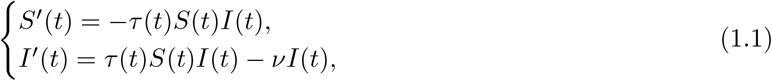
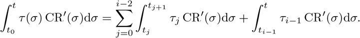
 In Figure 1, we compare the model to the COVID-19 data for mainland China. In order to estimate the parameter χ3, we minimize the distance between CRData(t)+ χ3 and the best exponential fit
 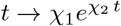 (i.e. we use the MATLAB function fit(t, data, ‘exp1’)).

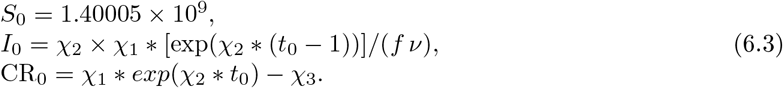
In this figure, we plot the best fit of the exponential model to the cumulative number of reported cases of COVID-19 in mainland China between February 19 and March 1. We obtain χ1 = 3.7366, χ2 = 0.2650 and χ3 = 615.41 with t0 = 19 Feb. The parameter χ3 is obtained by minimizing the error of the best fit exponential fit and the data.
The estimated initial number of infected and transmission rate


Fixing f = 0.5 and ν = 0.2, we obtain
 and
and
The influence of the errors made in the estimations (at the early stage of the epidemic) has been considered in the recent article by Roda et al. [20]. To understand this problem, let us first consider the case of the rate of transmission τ (t) = τ0 in the model (1.1). In that case (1.1) becomes
 By using the S-equation of model (2.6)
 where CI(t) is the cumulated number of infectious individuals. By replacing S(t) by this formula in I-equation of (2.6) we obtain
 Therefore, by taking the integral between t and t0 of the above equation, we obtain
 The equation (2.7) is indeed a monotone. We refer to Hal Smith [21] for a comprehensive presentation on the monotone systems. By applying a comparison principle to (2.7), we are in a position to confirm the intuition about epidemic SI models. Notice that the monotone properties are only true for the cumulative number of infectious (this is false for the number of infectious).
Let t > t0 be fixed. The cumulative number of infectious CI(t) is strictly increasing with respect to the following quantities
I0 > 0 the initial number of infectious individuals;
S0 > 0 the initial number of susceptible individuals;
τ > 0 the transmission rate;
1/ν > 0 the average duration of the infectiousness period.
Error in the estimated initial number of infected and transmission rate
Assume that the parameters χ1 and χ2 are estimated into an interval of confidence of 95% as
 and
and
 We obtain
 and
and

By using the data for mainland China we obtain

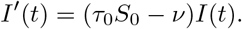
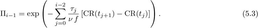
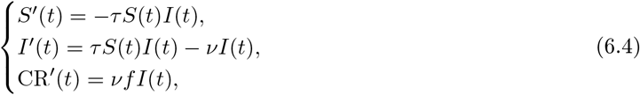
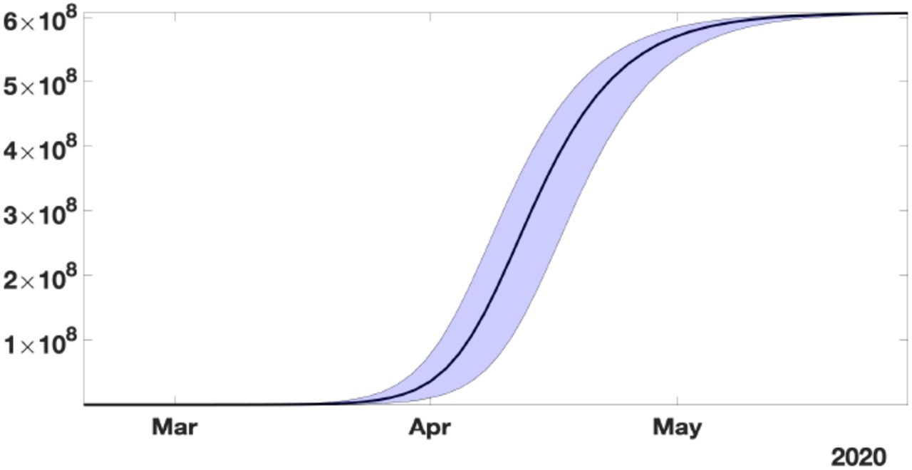
In Figure 2, we plot the upper and lower solutions CR+(t) (obtained by using 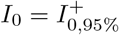 and
and  ) and CR−(t) (obtained by using
  and
and  ) corresponding to the blue region and the black curve corresponds to the best estimated value I0 = 1521 and τ0 = 3.3214 × 10⁻¹⁰.

In this figure, the black curve corresponds to the cumulative number of reported cases CR(t) obtained from the model (2.6) with CR′(t) = νf I(t) by using the values I0 = 1521 and τ0 = 3.32 × 10⁻¹⁰ obtained from our method and the early data from February 19 to March 1. The blue region corresponds the 95% confidence interval when the rate of transmission τ (t) is constant and equal to the estimated value τ0 = 3.32 × 10⁻¹⁰.
Recall that the final size of the epidemic corresponds to the positive equilibrium of (2.7)
 In Figure 2 the changes in the parameters I0 and τ0 (in (2.8)-(2.9)) do not affect significantly the final size.
3 Theoretical formula for τ (t)
By using the S-equation of model (1.1) we obtain
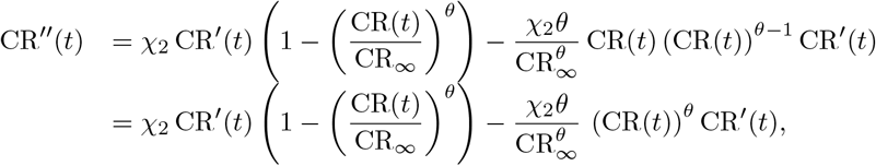
 next by using the I-equation of model (1.1) we obtain
 and by taking the integral between t and t0 we obtain Volterra’s integral equation for the cumulative number of infectious
 which is equivalent to (by using (1.3))
 The following result permit to obtains a perfect match between the SI model and the time-dependent rate of transmission τ (t).
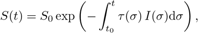
Let S0, ν, f, I0 > 0 and CR0 ≥ 0 be given. Let t → I(t) be the second component of system (1.1). Let  be a two times continuously differentiable function satisfying


 and
and
 Then
Then
 if and only if
 Proof. Assume first (3.7) is satisfied. Then by using equation (3.1) we deduce that
Therefore
 therefore by taking the derivative on both side
 and by using the fact that CR(t) − CR0 = νf CI(t) we obtain (3.8).
Conversely, assume that τ (t) is given by (3.8). Then if we define  and
and  , by using (3.3) we deduce that
 and by using (3.4)
 Moreover from (3.8) we deduce that Ĩ(t) satisfies (3.9). By using (3.10) we deduce that
  is a solution of (3.1). By uniqueness of the solution of (3.1), we deduce that
  ,∀t ≥ t0 or equivalently
  . The proof is completed.
The formula (3.8) was already obtained by Hadeler [19, see Corollary 2].
4 Explicit formula for τ (t) and I0
Many phenomenological models have been compared to the data during the first phase of the COVID-19 outbreak. We refer to the paper of Tsoularis and Wallace [22] a nice survey on the generalized logistic equations. Let us consider here for example, the Bernoulli-Verhulst’s equation
 supplemented with the initial data
 Let us recall the explicit formula for the solution of (4.1)
We assume that the cumulative numbers of reported cases CRData(ti) are known for a sequence of times t0 < t1 < … < tn+1.
Estimated initial number of infected
By combining (1.3) and the Bernoulli-Verhulst’s equation (4.1) for t → CR(t), we deduce the initial number of infected
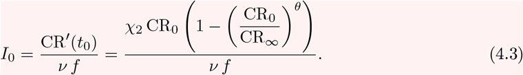
We fix f = 0.5, from the COVID-19 data in mainland China and formula (4.3) (with CR0 = 198), we obtain
 and
and
By using (4.1) we deduce that
 therefore

Estimated rate of transmission
By using the Bernoulli-Verhulst’s equation (4.1) and (4.4) replaced in (3.8), we
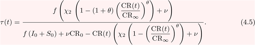 This formula (4.5) combined (4.2) gives an explicit formula for the rate of transmission.
Since CR(t) < CR∞, by considering the sign of the numerator and the denominator of (4.5), we obtain the following proposition.
The rate of transmission τ (t) given by (4.5) is non negative for all t ≥ t0 if
 and
and

Compatibility of the model SI with the COVID-19 data for mainland China
The model SI is compatible with the data only when τ (t) stays positive for all t ≥ t0. From our estimation of the Chinese’s COVID-19 data we obtain χ2 θ = 0.14. Therefore from (4.6) we deduce that model is compatible with data only when
 This means that the average duration of infectious period 1/ν must be shorter than 3.3 days.
Similarly the condition (4.7) implies
 and since we have CR0 = 198 and CR∞ = 67102, we obtain
 So according to this estimation the fraction of unreported 0 < f ≤ 1 can be almost as small as we want.
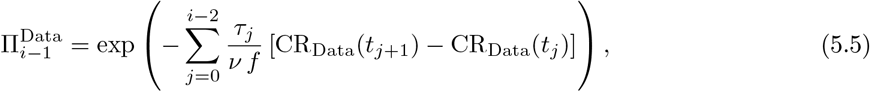
Figures 4 illustrates the Proposition 4.3. We observe that the formula for the rate of transmission (4.5) becomes negative whenever ν < χ2θ.

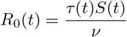
In this figure, we plot the best fit of the Bernoulli-Verhulst model to the cumulative number of reported cases of COVID-19 in China. We obtain χ2 = 0.66 and θ = 0.22. The black dots correspond to data for the cumulative number of reported cases and the blue curve corresponds to the model.

In this figure, we plot the rate of transmission obtained from formula (4.5) with f = 0.5, ν = 0.2 (in Figure (a)) and ν = 0.1 (in Figure (b)), χ2 = 0.66 and θ = 0.22 (i.e. χ2 θ = 0.14 < ν) and CR∞ = 67102 which is the latest value obtained from the cumulative number of reported cases for China.
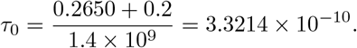
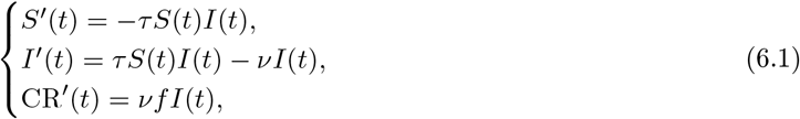
In Figure 5 we plot the numerical simulation obtain from (1.1)-(1.3) when t → τ (t) is replaced by the explicit formula (4.5). It is surprising that we can reproduce perfectly to the original Bernoulli-Verhulst even when τ (t) becomes negative. This was not guaranteed at first, since the I-class of individuals is losing some individuals which are recovering.

In this figure, we plot the number of reported cases by using model (1.1) and (1.3), and the rate of transmission is obtained in (4.5). The parameters values are f = 0.5, ν = 0.1 or ν = 0.2, χ2 = 0.66 and θ = 0.22 and CR∞ = 67102 is the latest value obtained from the cumulative number of reported cases for China. Furthermore, we use S0 = 1.4 × 10⁹ for the total population of China and I0 = 954 which is obtained from formula (4.3). The black dots correspond to data for the cumulative number of reported cases observed and the blue curve corresponds to the model.
5 Computing numerically a day by day piecewise constant rate of transmission
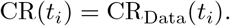
We assume that the rate of transmission τ (t) is piecewise constant and for each i = 0, …, n,

For t ∈ [ti−1, ti], we deduce by using Assumption 5.1 that
 Therefore by using (3.2), for t ∈ [ti−1, ti], we obtain
 where
where
 By fixing τi−1 = 0 on the right hand side of (5.2) we get
 and when τi−1 → ∞ we obtain
 By using the theory of monotone ordinary differential equations (see Smith [21]) we deduce that the map τi → CR(ti) is monotone increasing, and we get the following result.
Let assumptions 1.1, 4.1 and 5.1 be satisfied. Let I0 be fixed. Then we can find a unique sequence τ0, τ1, …, τn of non negative numbers such that t → CR(t) the solution of (3.2) fits exactly the data at any time ti, that is to say that
 if and only if the two following two conditions are satisfied for each i = 0, 1, …, n + 1,
 where
where
 and
and

The above theorem means that the data are identifiable for this model SI if and only if the conditions (5.4) and (5.6) are satisfied. Moreover, in that case, we can find a unique sequence of transmission rates τi ≥ 0 which gives a perfect fit to the data.
6 Numerical simulations
In this section, we propose a numerical method to fit the day by day rate of transmission. The goal is to take advantage of the monotone property of CR(t) with respect to τi on the time interval [ti, ti+1]. Recently more sophisticated methods were proposed by Bakha et al. [18] by using several types of approximation methods for the rate of transmission.
We start with the simplest Algorithm 1 in order to show the difficulties to identify the rate of transmission.
Step 1: We fix S0 = 1.4 × 10⁹, ν = 0.1 or ν = 0.2 and f = 0.5. We consider the system
 on the interval of time t ∈ [t0, t1]. This system is supplemented by initial values S(t0) = S0 and I(t0) = I0 is given by formula (2.4) (if we consider the data only at the early stage) or formula (4.3) (if we consider all the data) and CR(t0) = CRData(t0) obtained from the data.
The map τ → CR(t1) being monotone increasing, we can apply a bisection method the find the unique value τ0 solving
 Then we proceed by induction.
Step i: For each integer i = 1, …, n we consider the system
 on the interval of time t ∈ [ti, ti+1]. This system is supplemented by initial values S(ti) and I(ti) obtained from the previous iteration and with CR(ti) = CRData(ti) obtained from the data.
The map τ → CR(ti) being monotone increasing, we can apply a bisection method the find the value τi the unique value solving
In the numerical method we did not use the equation (5.2), because equation (5.2) is unstable numerically, while the original SI model behave relatively well numerically.
In Figure 6, we plot an example of such a perfect fit, which is the same for ν = 0.1 and ν = 0.2. In Figure 7 we plot the rate of transmission obtained numerically for ν = 0.2 in (a) and ν = 0.1 in (b). This is an example of a negative rate of transmission. Figure 7 should be compare to Figure 4 which gives similar result.

In this figure, we plot the perfect fit of the cumulative number of reported cases of COVID-19 in China. We fix the parameters f = 0.5 and ν = 0.2 or ν = 0.1 and we apply our algorithm 1 to obtain the perfect fit. The black dots correspond to data for the cumulative number of reported cases obtain and the blue curve corresponds to the model.

In this figure, we plot the rate of transmission obtained for the reported cases of COVID-19 in China with the parameters f = 0.5 and ν = 0.2 in figure (a) and ν = 0.1 in figure (b). This rate of transmission corresponds to the perfect fit obtained in Figure 6.
In Figures 8-10 we use Algorithm 1 and we plot the rate of transmission obtained by using the reported cases of COVID-19 in China where the parameters are fixed as f = 0.5 and ν = 0.2. In Figures 8-10, we observe an oscillating rate of transmission which is alternatively positive and negative back and forth. These oscillations are due to the amplification of the error in the numerical method itself. In Figure 8, we run the same simulation than in Figure 9 but during a shorter period. In Figure 8, we can see that the slope of CR(t) at the t = ti between two days (the black dots) is amplified one day to the next.

In figure (a), we plot the cumulative number of reported cases obtained from the data (black dots) and the model (blue curve). In figure (b), we plot the daily rate of transmission obtained by using Algorithm 1. We see that we can fit the data perfectly. But the method is very unstable. We obtain a rate of transmission that oscillates from the positive to the negative value back and forth.

In figure (a), we plot the cumulative number of reported cases obtained from the data (black dots) and the model (blue curve). In figure (b), we plot the daily rate of transmission obtained by using Algorithm 1. We see that we can fit the data perfectly. But the method being very unstable. We obtain a rate of transmission that oscillates from the positive to the negative value back and forth.
In Figure 10, we first smooth the original cumulative data by using the MATLAB function CRData = smoothdata(CRData, ′gaussian′, 50) to regularized the data and we apply Algorithm 1. Unfortunately, smoothing the data do not help to solve the instability problem in 10.

We apply Algorithm 1 the regularized data. In figure (a), we plot the regularized cumulative number of reported cases obtained from the data (black dots) and the model (blue curve). In figure (b), we plot the daily rate of transmission obtained by using Algorithm 1. We see that we can fit the data perfectly. But the method is very unstable. We obtain a rate of transmission that oscillates from the positive to the negative value back and forth.
We need to introduce a correction when choosing the next initial value I(ti). In Algorithm 1 the errors are due to the following relationship which is not respected
 at the points t = ti which should be reflected by the algorithm. In Figure 11, we smooth the data first by using the MATLAB function CRData= smoothdata(CRData, ′gaussian′, 50), and we apply Algorithm 2. We no longer observe the oscillations of the rate of transmission.

In this figure, we plot the rate of transmission obtained by using the reported cases COVID-19 in China with the parameters f = 0.5 and ν = 0.2. We first regulatized the data by applying the MATLAB function CRData = smoothdata(CRData, ′gaussian′, 50). Then we apply Algorithm 2 the regularized data. In figure (a), we plot the regularized cumulative number of reported cases obtained (black dots) and the model (blue curve). In figure (b), we plot the daily rate of transmission obtained by using the Algorithm 2. We see that we can fit the data perfectly and this time the rate of transmission is becoming reasonable.
Step 1: We fix S0 = 1.4 × 10⁹, ν = 0.1 or ν = 0.2 and f = 0.5. Then we fit the data by using the method described in Section 2 to estimate the parameters χ1, χ2 and χ3 from the day 1 to 10. Then we use
 For each integer i = 0, …, n, we consider the system
 for t ∈ [ti, ti+1]. Then the map τ → CR(ti+1) being monotone increasing, we can apply a bisection method to find the unique τi solving
 The key idea of this new Algorithm is the following correction on the I-component of the system. We start a new step by using the value S(ti) obtained from the previous iteration and

7 Discussion
In this article, we develop several method to understand how to reconstruct the rate of transmission from the data. In section 2, we reconsidered the method presented in [16] based in exponential fit of the early data. The approach gives a first estimation I0 and τ0. In Section 3, we prove a result to connect the time dependent cumulative reported data and the transmission rate. In Section 4, we compare the data to the Bernoulli-Verhulst model and we use this model as a phenomenological model. The Bernoulli-Verhulst model fit very well the data for mainland China. Next by replacing the data by the solution of the Bernoulli-Verhulst model, we obtain an explicit formula for the transmission. So we derive some condition on the parameters for the applicability of the SI model to the data for mainland China. In Section 5, we discretized the rate of transmission and we observe that given some daily cumulative data, we can get at most one perfect fit the data. Therefore, in Section 6, we provide two algorithm to compute numerically the daily rates of transmission. Such a numerical questions turns to be a delicate problem. This problem was previously considered by another French group Bakhta, Boiveau, Maday and Mula [18]. Here we use some simple idea to approach the derivative of the cumulative reported cases combined with some smoothing method applied to the data.
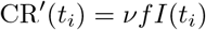
To conclude this article we plot the daily basic reproduction number
 in function of the time t and the parameters f or ν. This above simple formula for R0 is not the real basic reproductive number in the sense of the number of newly infected produced by a single infectious. But this is a simple formula which gives a good tenancy about the growth or decay of the number of infectious. In Figure 12-(a), the daily basic reproduction number is almost independent of f, while in Figure 12-(b), R0(t) is depending on ν mostly for the small value of ν. The red curve on each surfaces in Figure 12 correspond to the turning point (i.e. time t ≥ t0 for which R0(t) = 1). We also see that turning point is not depending much on these parameters.

In this figure plot 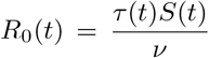 the daily basic reproduction number and we vary the parameter f (top) and ν (bottom).
Concerning contagious diseases, public health physicians are constantly faced with four challenges. The first concerns the estimation of the average transmission rate. Until now, no explicit formula had been obtained, in the case of the SIR model, according to the observed data of the epidemic, that is to say the number of reported cases of infected patients. Here, from realistic simplifying assumptions, a formula is provided (formula (4.5)), making it possible to accurately reconstruct theoretically the curve of the observed cumulative cases. The second challenge concerns the estimation of the mean duration of the infectious period for infected patients. As for the transmission rate, the same realistic assumptions make it possible to obtain an upper limit to this duration (inequality (4.8)), which makes it possible to better guide the individual quarantine measures decided by the authorities in charge of public health. This upper bound also makes it possible to obtain a lower bound for the percentage of unreported infected patients (inequality (4.8)), which gives an idea of the quality of the census of cases of infected patients, which is the third challenge facing epidemiologists, specialists of contagious diseases. The fourth challenge is to the estimation of the average transmission rate for each day of the infectious period (dependent on the distribution of the transmission over the “ages” of infectivity), which will be the subject of further work and which poses formidable problems, in particular those related to the age (biological age or civil age) class of the patients concerned. Another interesting prospect is the extension of methods developed in the present paper to the contagious non-infectious diseases (i.e., without causal infectious agent), such as social contagious diseases, the best example being that of the pandemic linked to obesity [23, 24, 25], for which many concepts and modeling methods remain available.
Data Availability
The data used are available from internet
Funding
This research was funded by the Agence Nationale de la Recherche in France (Project name : MPCUII (PM)).
Conflicts of Interest
Declare conflicts of interest or state “The authors declare no conflict of interest.”


