
Abstract
The COVID-19 pandemic has created a public health crisis. Because SARS-CoV-2 can spread from individuals with pre-symptomatic, symptomatic, and asymptomatic infections [1, 2, 3], the re-opening of societies and the control of virus spread will be facilitated by robust surveillance, for which virus testing will often be central. After infection, individuals undergo a period of incubation during which viral titers are usually too low to detect, followed by an exponential growth of virus, leading to a peak viral load and infectiousness, and ending with declining viral levels and clearance [4]. Given the pattern of viral load kinetics [4], we model surveillance effectiveness considering test sensitivities, frequency, and sample-to-answer reporting time. These results demonstrate that effective surveillance, including time to first detection and outbreak control, depends largely on frequency of testing and the speed of reporting, and is only marginally improved by high test sensitivity. We therefore conclude that surveillance should prioritize accessibility, frequency, and sample-to-answer time; analytical limits of detection should be secondary.
The reliance on testing as a means to safely reopen societies has placed a microscope on the analytical sensitivity of virus assays, with a gold-standard of quantitative real-time polymerase chain reaction (qPCR). These assays have analytical limits of detection that are usually within around 103 viral RNA copies per ml (cp/ml) [5]. However, qPCR remains expensive and as a laboratory based assay often have sample-to-result times of 24-48 hours. New developments in SARS-CoV-2 diagnostics have the potential to reduce cost significantly, allowing for expanded testing or greater frequency of testing and can reduce turnaround time to minutes. These assays however largely do not meet the gold standard for analytical sensitivity, which has encumbered translation of these assays for widescale use [6].
Three features of the viral increase, infectivity, and decline during SARS-CoV-2 infection led us to hypothesize that there might be minimal differences in effective surveillance using viral detection tests of different sensitivities, such as RT-qPCR with a limit of detection (LOD) at 103 cp/ml [5] compared to often cheaper or faster assays with higher limits of detection (i.e., around 105 cp/ml) such as point-of-care nucleic acid LAMP and rapid antigen tests (Figure 1A). First, since filtered samples collected from patients displaying less than 106 N or E RNA cp/ml contain minimal or no measurable infectious virus [7, 8, 9], either class of test should detect individuals who are currently infectious. The absence of infectious particles at viral RNA concentrations < 106 cp/ml is likely due to (i) the fact that the N and E RNAs are also present in abundant subgenomic mRNAs, leading to overestimation of the number of actual viral genomes by ∼ 100-1000X [10], (ii) technical artifacts of RT-PCR at Ct values > 35 due to limited template [11, 12], and (iii) the production of non-infectious viral particles as is commonly seen with a variety of RNA viruses [13]. Second, during the exponential growth of the virus, the time difference between 103 and 105 cp/ml is short, allowing only a limited window in which only the more sensitive test could diagnose individuals. For qPCR, this corresponds to the time required during viral growth to go from Ct values of 40 to ∼ 34. While this time window for SARS-CoV-2 is not yet rigorously defined, for other respiratory viruses such as influenza, and in ferret models of SARS-CoV-2 transmission, it is on the order of a day [14, 15]. Finally, high-sensitivity screening tests, when applied during the viral decline accompanying recovery, are unlikely to substantially impact transmission because such individuals detected have low, if any, infectiousness [10].
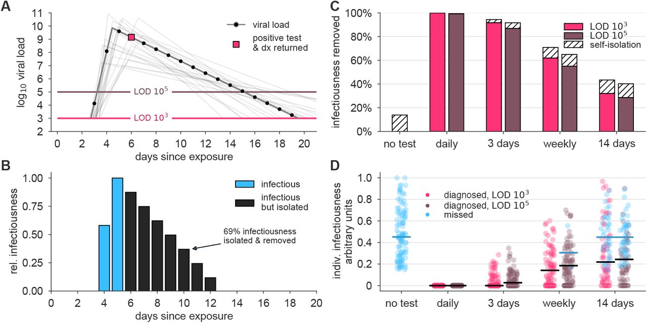
(A) An example viral load trajectory is shown with LOD thresholds of two tests, and a hypothetical positive test on day 6, two days after peak viral load. 20 other stochastically generated viral loads are shown to highlight trajectory diversity (light grey; see Methods). (B) Relative infectiousness for the viral load shown in panel A pre-test, totaling 31% (blue) and post-isolation, totaling 69% (black). (C) Surveillance programs using tests at LODs of 103 and 105 at frequencies indicated were applied to 10, 000 individuals trajectories of whom 20% would undergo symptomatic isolation near their peak viral load if they had not been tested and isolated first. Total infectiousness removed during surveillance (colors) and self isolation (hatch) are shown for surveillance as indicated, relative to total infectiousness with no surveillance or self-isolation. (D) The impact of surveillance on the infectiousness of 100 individuals is shown for each surveillance program and no testing, as indicated, with each individual colored by test if their infection was detected during infectiousness (medians, black lines) or colored blue if their infection was missed by surveillance or detected positive after their infectious period (medians, blue lines). Units are arbitrary and scaled to the maximum infectiousness of sampled individuals.
To examine how surveillance testing would reduce the average infectiousness of individuals, we first modeled the viral loads and infectiousness curves of 10,000 simulated individuals using the predicted viral trajectories of SARS-CoV-2 infections based on key features of latency, growth, peak, and decline identified in the literature (Figure 1A; see Methods). Accounting for these within-host viral kinetics, we calculated what percentage of their total infectiousness would be removed by surveillance and isolation (Figure 1B) with tests at LOD of 103 and 105, and at different frequencies. Here, infectiousness was taken to be proportional to the logarithm of viral load (with alternative assumptions addressed in Supplemental Materials), consistent with the observation that pre-symptomatic patients are most infectious just prior to the onset of symptoms [4], and evidence that the efficiency of viral transmission coincides with peak viral loads, which was also identified during the related 2003 SARS outbreak [16, 17]. We considered that 20% of patients would undergo symptomatic isolation near their peak viral load if they had not been tested and isolated first, and 80% would have sufficiently mild or no symptoms such that they would not isolate unless they were detected by surveillance testing. This analysis demonstrated that there was little difference in averting infectiousness between the two classes of test. Dramatic reductions in total infectiousness of the individuals were observed by testing daily or every third day, ∼ 60% reduction when testing weekly, and < 40% under biweekly testing (Figure 1C). Because viral loads and infectiousness vary across individuals, we also analyzed the impact of different surveillance regimes on the distribution of individuals’ infectiousness (Figure 1D).
Above, we assumed that each infection was independent. To investigate the effects of surveillance testing strategies at the population level, we used simulations to monitor whether epidemics were contained or became uncontrolled, while varying the frequencies at which the test was administered, ranging from daily testing to testing every 14 days, and considering tests with LOD of 103 and 105, analogous to RT-qPCR and RT-LAMP / rapid antigen tests, respectively. We used two different epidemiological models to ensure that important observations were independent of the specific modeling approach. The first model is a previously described agent-based model with both within-household and age-stratified contact structure based on census microdata in a city representative of New York City [18], and initialized with 100 cases without additional external infections. The second model is a simple fully mixed model representing a population of 20,000, similar to a large university setting, with a constant rate of external infection approximately equal to one new import per day. Individual viral loads were simulated for each infection, and individuals who received a positive test result were isolated, but contact tracing and monitoring was not included to more conservatively estimate the impacts of surveillance alone [19, 20]. Model details and parameters are fully described in Methods.
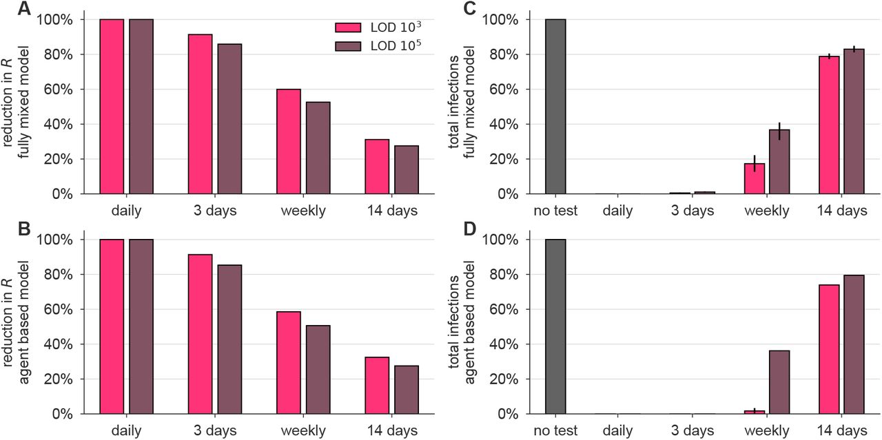
We observed that a surveillance program administering either test with high frequency limited viral spread, measured by both a reduction in the reproductive number R (Figures 2A and B; see Methods for calculation procedure) and by the total infections that persisted in spite of different surveillance programs, expressed relative to no surveillance (Figures 2C and D). Testing frequency was found to be the primary driver of population-level epidemic control, with only a small margin of improvement provided by using a more sensitive test. Direct examination of simulations showed that with no surveillance or biweekly testing, infections were uncontrolled, whereas surveillance testing weekly with either LOD = 103 or 105 effectively attenuated surges of infections (examples shown in Figure S1).

Both the fully-mixed compartmental model (top row) and agent based model (bottom row) are affected by surveillance programs. (A, B) More frequent testing reduces the effective reproductive number R, shown as the percentage by which R0 is reduced, 100 × (R0− R)/R0. Values of R were estimated from 50 independent simulations of dynamics (see Methods). (C, D) Relative to no testing (grey bars), surveillance suppresses the total number of infections in both models when testing every day or every three days, but only partially mitigates total cases for weekly or bi-weekly testing. Error bars indicate inner 95% quantiles of 50 independent simulations each.
The relationship between test sensitivity and the frequency of testing required to control outbreaks in both the fully mixed model and the agent-based model generalize beyond the examples shown in Figure 2 and are also seen at other testing frequencies and sensitivities. We simulated both models at LODs of 103, 105, and 106, and for testing ranging from daily to every 14 days. For those, we measured each surveillance policy’s impact on total infections (Figure S2A and B) and on R (Figure S2C and D). In Figure 2, we modeled infectiousness as proportional to log10 of viral load. To address whether these finding are sensitive to this modeled relationship, we performed similar simulations with infectiousness proportional to viral load (Figure S3), or uniform above 106/ml (Figure S4). We found that results were robust to these large variations in the modeled relationship between infectiousness and viral load.
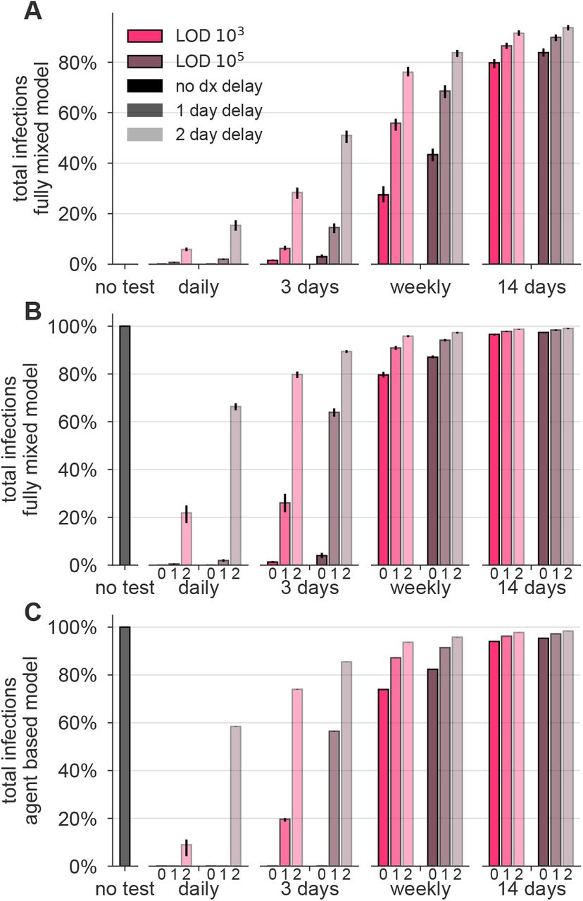
An important variable in surveillance testing is the time between a test’s sample collection and the reporting of a diagnosis. To examine how time to reporting affected epidemic control, we re-analyzed both the reduction in individuals’ infectiousness, as well as the epidemiological simulations, comparing the results of instantaneous reporting (reflecting a rapid point-of-care assay), one day delay, and two day delay (Figure 3A and B). Delays in reporting dramatically decreased the reduction in infectiousness in individuals as seen by the total infectiousness removed (Figure 3C), the distribution of infectiousness in individuals (Figure 3D), or the dynamics of the epidemiological models (Figure 4). This result was robust to the modeled relationship between infectiousness and viral load in both simulation models and for various test sensitivities and frequencies (Figure S5). These results highlight that delays in reporting lead to dramatically less effective control of viral spread and emphasize that fast reporting of results is critical in any surveillance testing. These results also reinforce the relatively smaller benefits of improved limits of detection.
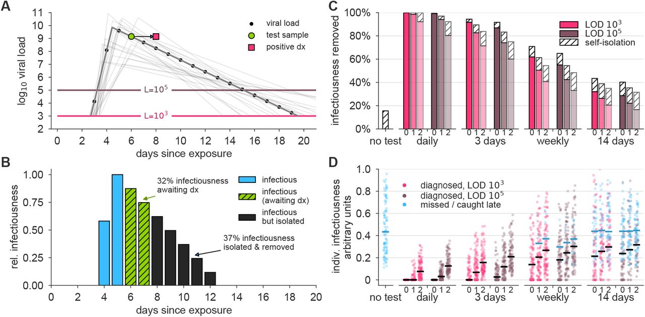
(A) An example viral load trajectory is shown with LOD thresholds of two tests, and a hypothetical positive test on day 6, but with results reported on day 8. 20 other stochastically generated viral loads are shown to highlight trajectory diversity (light grey; see Methods). (B) Relative infectiousness for the viral load shown in panel A pre-test (totaling 31%; blue) and post-test but pre-diagnosis (totaling 32%; green), and post-isolation (totaling 37%; black). (C) Surveillance programs using tests at LODs of 103 and 105 at frequencies indicated, and with results returned after 0, 1, or 2 days (indicated by small text beneath bars) were applied to 10, 000 individuals trajectories of whom 20% were symptomatic and self-isolated after peak viral load if they had not been tested and isolated first. Total infectiousness removed during surveillance (colors) and self isolation (hatch) are shown, relative to total infectiousness with no surveillance or self-isolation. Delays substantially impact the fraction of infectiousness removed. (D) The impact of surveillance with delays in returning diagnosis of 0, 1, or 2 days (small text beneath axis) on the infectiousness of 100 individuals is shown for each surveillance program and no testing, as indicated, with each individual colored by test if their infection was detected during infectiousness (medians, black lines) or colored blue if their infection was missed by surveillance or diagnosed positive after their infectious period (medians, blue lines). Units are arbitrary and scaled to the maximum infectiousness of sampled individuals.

The effectiveness of surveillance programs are dramatically diminished by delays in reporting in both the fully-mixed compartmental model (top row) and agent based model (bottom row). (A, B) The impact of surveillance every day, 3 days, weekly, or biweekly, on the reproductive number R, calculated as 100 × (R0 − R)/R0, is shown for LODs 103 and 105 and delays of 0, 1, or 2 days (small text below axis). Values of R were estimated from 50 independent simulations of dynamics (see Methods). (C, D) Relative to no testing (grey bars), surveillance suppresses the total number of infections in both models when testing every day or every three days, but delayed results lead to only partial mitigation of total cases, even for testing every day or 3 days. Error bars indicate inner 95% quantiles of 50 independent simulations each.
Communities vary in their transmission dynamics, due to difference in rates of imported infections and in the basic reproductive number R0, both of which will influence the frequency and sensitivity with which surveillance testing must occur. We performed two analyses to illustrate this point. First, we varied the rate of external infection in our fully mixed model, and confirmed that when the external rate of infection is higher, more frequent surveillance is required to prevent outbreaks (Figure S6A). Second, we varied the reproductive number R0 between infected individuals in both models, and confirmed that at higher R0, more frequent surveillance is also required (Figure S6B and C). This may be relevant to institutions like college campuses or military bases wherein frequent classroom setting or dormitory living are likely to increase contact rates. Thus, the specific strategy for successful surveillance will depend on the current community infection prevalence and transmission rate.
Our results lead us to conclude that surveillance testing of asymptomatic individuals can be used to limit the spread of SARS-CoV-2. However, our findings are subject to a number of limitations. First, the sensitivity of a test may depend on factors beyond LOD, including manufacturer variation and improper clinical sampling [21], though the latter may be ameliorated by different approaches to sample collection, such as saliva-based testing [22]. Second, the exact performance differences between testing schemes will depend on whether our model truly captures viral kinetics and infectiousness profiles [4], particularly during the acceleration phase between exposure and peak viral load. Continued clarification of these within-host dynamics would increase the impact and value of this, and other [19, 20] modeling studies.
A critical point is that the requirements for surveillance testing are distinct from clinical testing. Clinical diagnoses target symptomatic individuals, need high accuracy and sensitivity, and are not limited by cost. Because they focus on symptomatic individuals, those individuals can isolate such that a diagnosis delay does not lead to additional infections. In contrast, results from the surveillance testing of asymptomatic individuals need to be returned quickly, since even a single day diagnosis delay compromises the surveillance program’s effectiveness. Indeed, at least for viruses with infection kinetics similar to SARS-CoV-2, we find that speed of reporting is much more important than sensitivity, although more sensitive tests are nevertheless somewhat more effective.
The difference between clinical and surveillance testing highlights the need for additional tests to be approved and utilized for surveillance. Such tests should not be held to the same degree of sensitivity as clinical tests, in particular if doing so encumbers rapid deployment of faster cheaper SARS-CoV-2 assays. We suggest that the FDA, other agencies, or state governments, encourage the development and use of alternative faster and lower cost tests for surveillance purposes, even if they have poorer limits of detection. If the availability of point-of-care or self-administered surveillance tests leads to faster turnaround time or more frequent testing, our results suggest that they would have high epidemiological value.
Our modeling suggests that some types of surveillance will subject some individuals to unnecessary quarantine days. For instance, the infrequent use of a sensitive test will not only identify (i) those with a low viral load in the beginning of the infection, who must be isolated to limit viral spread, but (ii) those in the recovery period, who still have detectable virus or RNA but are below the infectious threshold [9, 10]. Isolating this second group of patients will have no impact on viral spread but will incur costs of isolation. The use of serology, repeat testing 24 or 48 hours apart, or some other test, to distinguish low viral load patients on the upslope of infection from those in the recovery phase could allow for more effective quarantine decisions.
Data Availability
Simulation code is available via GitHub.
Supplemental Figures and Tables

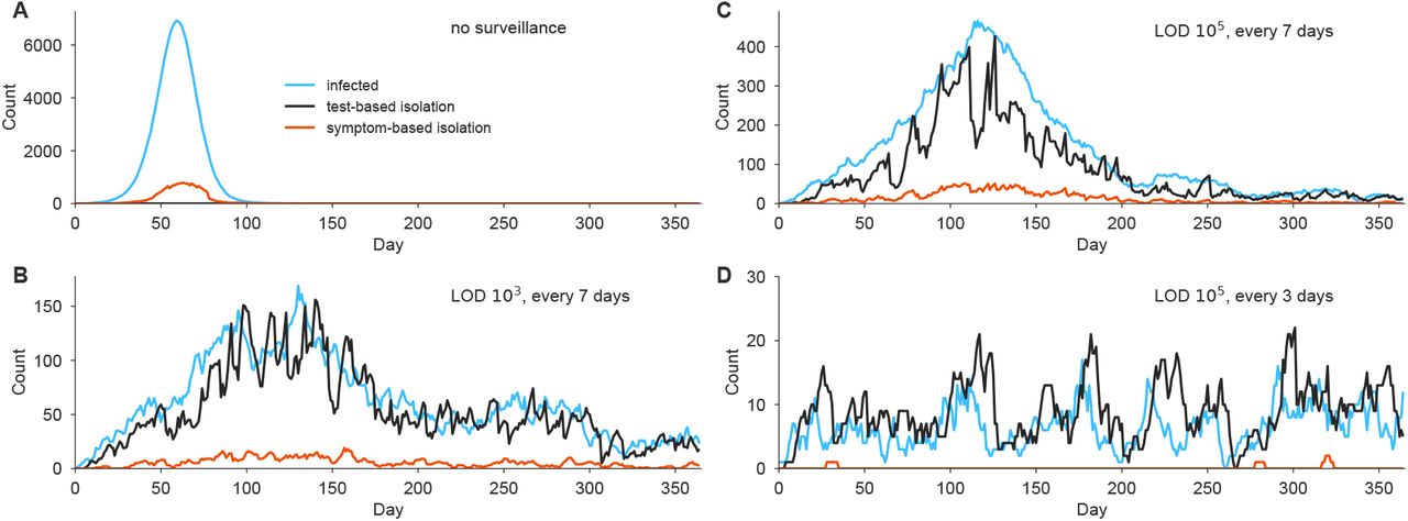
Simulation trajectories show the number of infected individuals in a population of N = 20, 000 with a constant rate of external infection set to 1/N per person per day, i.e. around 1 imported case per day. Infections (blue), test-based isolation (black), and symptom-based isolation (red) are shown for four scenarios, with R0 = 2.5. (A) No surveillance. (B) Weekly testing at LOD 103. (C) Weekly testing at LOD 105. (D) Testing every 3 days with LOD 105. Note the variation in the vertical axis scales. The model is fully described in Methods.

The fully mixed model (top row) and agent based model (bottom row) were simulated (Methods) with various test frequencies, ranging from daily to once every 14 days, and with LODs of 103, 105, and 106. Modeling results show mean outcomes from 50 independent simulations at each point, expressed as (A, B) total infections and (C, D) effective reproductive number R, from a baseline of R0 = 2.5. For the fully mixed model, only secondary infections are shown, excluding imported infections. Total population sizes were N = 2 × 10⁴ for the fully mixed model and 8.4 × 10⁶ for the agent based model. Dashed lines indicate R = 1 for reference.

This figure presents results from simulations which were identical to those shown in the main text Figure 4, but in which infectiousness was assumed to be directly proportional to viral load. Compare with threshold (binary) infectiousness in Fig. S4 and log-proportional infectiousness in Fig 4. See Methods.

This figure presents results from simulations which were identical to those shown in the main text Figure 4, but in which infectiousness was assumed to be binary, i.e. no infectiousness below 106 and equal infectiousness for any viral load above 106. Compare with proportional infectiousness in Fig. S3 and log-proportional infectiousness in Fig 4. See Methods.

The fully mixed model and agent based model were simulated (Methods) with various test frequencies, ranging from daily to once every 14 days, with LODs of 103, 105, and 106, and with delays of 0, 1, 2, or 3 days, for log-proportional, proportional, and threshold infectiousness functions (see Methods). Legends in panels A and B indicate LODs and delays, and in-plot annotations describe various conditions. Modeling results show mean outcomes from 50 independent simulations at each point, expressed as total infections and effective reproductive number R, from a baseline of R0 = 2.5. For the fully mixed model, only secondary infections are shown, excluding imported infections. Total population sizes were N = 2 × 10⁴ for the fully mixed model and 8.4 × 10⁶ for the agent based model. Dashed lines indicate R = 1 for reference.

(A) Results from the fully-mixed simulation with a tripled rate of external infection, i.e. 3/N per person per day. (B) Results from the fully mixed simulation with R0 doubled, i.e. R0 = 5. (C) Results from the agent-based simulation with R0 doubled, i.e. R0 = 5.

Example viral load (line) with stochastic control points highlighted (squares). Because simulations took place in discrete time, dots show points at which this example viral load would have been sampled. Light grey lines show 20 alternative trajectories to illustrate the diversity of viral loads drawn from the simple model.
Methods
Viral Loads
Viral loads were drawn from a simple viral kinetics model intended to capture (1) a variable latent period, (2) a rapid growth phase from the lower limit of PCR detectability to a peak viral load, and (3) a slower decay phase. These dynamics were based on the following observations.
Latent periods prior to symptoms have been estimated to be around 5 day [23]. Viral load appears to peak prior to symptom onset [4], and peaks within 2 days of challenge in a macaque model [24, 25], though it should be noted that macaque challenge doses were high. Viral load decreases monotonically from the time of symptom onset [4, 26, 27, 28, 29], but may be high and detectable 3 or more days before symptom onset [1, 30]. Peak viral loads are difficult to measure due to lack of prospective sampling studies of individuals prior to exposure and infection, but viral loads have been reported in the range of 𝒪 (104) to 𝒪 (109) copies per ml [8, 28, 29]. Viral loads appear to become undetectable by PCR within 3 weeks of symptom onset [26, 29, 31], but detectability and timing may differ depending on the degree or presence of symptoms [31, 32]. Finally, we note that the general understanding of viral kinetics may vary depending on the mode of sampling, as demonstrated via a comparison between sputum and swab samples [8].
To mimic growth and decay, log10 viral loads were specified by a continuous piecewise linear “hinge” function, specified uniquely with three control points: (t0, 3), (tpeak, Vpeak),(tf, 6) (Figure S7; green squares). The first point represents the time at which an individual’s viral load first crosses 103, with t0∼ unif[2.5, 3.5], measured in days since exposure. The second point represents the peak viral load. Peak height was drawn Vpeak∼ unif[7, 11], and peak timing was drawn with respect to the start of the exponential growth phase, tpeak −t0∼ 0.2 + gamma(1.8). The third point represents the time at which an individual’s viral load crosses beneath the 106 threshold, at which point viral loads no longer cause active cultures in laboratory experiments [], and was drawn with respect to peak timing, tf −tpeak ∼ unif[5, 10]. In simulations, each viral load’s parameters were drawn independently of others, and the continuous function described here was evaluated at 21 integer time points (Figure S7; black dots) representing a three week span of viral load values.
Infectiousness
Infectiousness F was assumed to be directly related to viral load V in one of three ways. In the main text, each individual’s relative infectiousness was proportional log10 of viral load’s excess beyond 106, i.e. F ∝ log10(V) − 6. In the supplementary sensitivity analyses, we investigated two opposing extremes. To capture a more extreme relationship between infectiousness and viral load, we considered F to be directly proportional to viral load’s excess above 106, i.e.  , and to capture a more extreme relationship, but in the opposing direction, we considered F to simply be a constant when viral load exceeded 106, i.e.
 . We call these three functions log-proportional, proportional, and threshold throughout the text and supplemental materials.
Recently, He et al [4] published an analysis of infectiousness relative to symptom onset. Among our infectiousness functions, this inferred relationship bears the greatest similarity, over time, to the log-proportional infectiousness function, as visualized in Figs. 1 and 3. The proportional and threshold models therefore represent one of many types of sensitivity analysis. Results for those models can be found in Figures S3, S4, and S5.
In all simulations, the value of the proportionality constant implied by the infectiousness functions above was chosen to achieve the targeted value of R0 for that simulation, and confirmed via simulation as described below.
Disease Transmission Models
Overview
Two models were used to simulate SARS-CoV-2 dynamics, both based on a typical compartmental framework. The first model was a fully-mixed model of N = 20, 000 individuals with all-to-all contact structure, zero initial infections, and a constant 1/N per-person probability of becoming infected from an external source. This model could represent, for instance, a large college campus with high mixing, situated within a larger community with low-level disease prevalence. The second model was an agent-based model of N = 8.4 million agents representing the population and contact structure of New York City, as previously described [18]. Contact patterns were based on a combination of individual-level household contacts drawn from census microdata and age-stratified contact matrices which describe outside of household contacts. This model was initialized with 100 initial infections and no external sources of infection.
Both the fully-mixed and agent-based models tracked discrete individuals who were Susceptible (S), Infected (I), Recovered (R), Isolated (Q), and Self-Isolated (SQ) at each discrete one day timestep. Upon becoming infected (S→I), a viral load trajectory V (t) was drawn which included a latent period, growth, and decay. Each day, an individual’s viral load trajectory was used to determine whether their diagnostic test would be positive if administered, as well as their infectiousness to susceptible individuals. Based on a schedule of testing each person every D days, if an individual happened to be tested on a day when their viral load exceeded the limit of detection L of the test, their positive result would cause them to isolate (I → Q), but with the possibility of a delay in turnaround time. A fraction 1− f of individuals self-isolate on the first day after peak viral load, to mimic symptom-driven isolation (I → SQ), with f = 0.8 for the fully mixed model and f = 1 for the agent based model. When an individual’s viral load dropped below 103, that individual recovered (I, Q, SQ → R). Details follow.
Testing, Isolation, and Sample-to-Answer Turnaround Times
All individuals were tested every D days, so that they could be moved into isolation if their viral load exceeded the test’s limit of detection V (t) > L. Each person was deterministically tested exactly every D days, but testing days were drawn uniformly at random such that not all individuals were tested on the same day. To account for delays in returning test results, we included a sample-to-answer turnaround time T, meaning that an individual with a positive test on day t would isolate on day t + T.
Transmission, Population Structure, and Mixing Patterns: Fully-mixed model
Simulations were initialized with all individuals susceptible, S = N. Each individual was chosen to be symptomatic independently with probability f, and each individual’s first test day (e.g. the day of the week that their weekly test would occur) was chosen uniformly at random between 1 and D. Relative infectiousness was scaled up or down to achieve the specified R0 in the absence of any testing policy, but inclusive of any assumed self-isolation of symptomatics.
In each timestep, those individuals who were marked for testing that day were tested, and a counter was initialized to T, specifying the number of days until that individual received their results. Next, individuals whose test results counters were zero were isolated, I → Q. Then, symptomatic individuals whose viral load had declined relative to the previous day were self-isolated, I→SQ. Next, each susceptible individual was spontaneously (externally) infected independently with probability 1/N, S → I. Then, all infected individuals contacted all susceptible individuals, with the probability of transmission based on that day’s viral load V (t) for each person and the particular infectiousness function, described above, S → I.
To conclude each time step, individuals’ viral loads and test results counters were advanced, with those whose infectious period had completely passed moved to recovery, I, Q, SQ → R.
Transmission, Population Structure, and Mixing Patterns: Agent-based model
The agent-based model added viral kinetics and testing policies (as described above) to an existing model for SARS-CoV-2 transmission in New York City. A full description of the agent-based model is available [18]; here we provide an overview of the relevant transmission dynamics.
Simulations were initialized with all individuals susceptible, except for 100 initially infected individuals, S = N − 100. As in the fully-mixed model, each individual’s test day was chosen uniformly at random and relative infectiousness was scaled to achieve the specified R0.
In each timestep, those individuals who were marked for testing that day were tested, and a counter was initialized to T, specifying the number of days until that individual received their results. Next, individuals whose test results counters were zero were isolated, I→Q. There was no self-isolation in this model (and accordingly, the model did not label individuals as symptomatic or asymptomatic).
Then, transmission from infected individuals to susceptible individuals was simulated both within and outside households. To model within-household transmission, each individual had a set of other individuals comprising their household. Household structures, along with the age of each individual, were sampled from census microdata for New York City [33]. The probability for an infectious individual to infect each of their household members each day was determined by scaling the relative infectiousness values to match the estimated secondary attack rate for close household contacts previously reported in case cluster studies [34].
Outside of household transmission was simulated using age-stratified contact matrices, which describe the expected number of daily contacts between an individual in a given age group and those in each other age group. Each infectious individual of age i drew Poisson(Mij) contacts with individuals in age group j, where M is the contact matrix. The contacted individuals were sampled uniformly at random from age group j. We use a contact matrix for the United States estimated by [35]. Each contact resulted in infection, S→ I, with probability proportional to the relative infectiousness of the infected individual on that day, scaled to obtain the specified value of R0.
To conclude each time step, individuals’ viral loads and test results counters were advanced, with those whose infectious period had completely passed moved to recovery, I, Q → R.
Calibration to achieve targeted R0 and estimation of R
As a consistency check, each simulation’s R0 was estimated as follows, to ensure that simulations were properly calibrated to their intended values. Note that to vary R0, the proportionality constant in the function that maps viral load to infectiousness need only be adjusted up or down. In a typical SEIR model, this would correspond to changing the infectiousness parameter which governs the rate at which I-to-S contacts cause new infections β.
For the fully-mixed, the value of R0 was numerically estimated by running single-generation simulations in which a 50 infected individual were placed in a population of N − 50 others. The number of secondary infections from those initially infected was recorded and used to directly estimate R0.
For the agent-based model, the value of R0 depends on the distribution of infected agents due to stratification by age and household. We numerically estimate R0 by averaging over the number of secondary infections caused by each agent who was infected in the first 15 days of the simulation (at which point the population is still more than 99.99% susceptible).
Estimations of R proceeded exactly as estimations of R0 for both models, except with interventions applied to the the viral loads and therefore the dynamics.
Acknowledgements
The authors wish to thank the BioFrontiers Institute IT HPC group. This work was supported by grants NIH F32 AI145112 (James Burke), NIH F30 AG063468 (Evan Lester), MURI W911NF-17-1-0370 (Milind Tambe), an NIH directors DP5 award 1DP5OD028145-01 (Michael Mina), and the Howard Hughes Medial Institute (Roy Parker).


