
Abstract
In response to the COVID-19 pandemic, many higher educational institutions moved their courses on-line in hopes of slowing disease spread. The advent of multiple highly-effective vaccines offers the promise of a return to “normal” in-person operations, but it is not clear if – or for how long – campuses should employ non-pharmaceutical interventions such as requiring masks or capping the size of in-person courses. In this study, we develop and fine-tune a model of COVID-19 spread to UC Merced’s student and faculty population. We perform a global sensitivity analysis to consider how both pharmaceutical and non-pharmaceutical interventions impact disease spread. Our work reveals that vaccines alone may not be sufficient to eradicate disease dynamics and that significant contact with an infected surrounding community will maintain cases on-campus. Our work provides a foundation for higher-education planning allowing campuses to balance the benefits of in-person instruction with the ability to quarantine/isolate infected individuals.
1 Introduction
In late 2019, a novel coronavirus, SARS-CoV-2, was identified as the cause of a cluster of pneumonia cases [1]. On March 11, 2020 the World Health Organization declared the 2019 novel coronavirus outbreak (COVID-19) a pandemic [2]. Shortly after, nearly every higher-education institute rapidly transitioned all classes to on-line instruction to “flatten the epidemic curve”. As of February 8, 2022 the cumulative number of confirmed COVID-19 cases exceeds 400 million [3]. Although the advent of multiple effective vaccines offers the likelihood of a return to normal life, with the advent of booster shots and the emergence of highly-infectious variants means that the return to our pre-COVID existence is not in our immediate future [4].
In Fall 2020 in the United States, many colleges and universities attempted to re-open their class-rooms and dorms to students with mixed-results. Overall, there were substantial increases in the number of new COVID-19 cases after school re-opening [5]. Moreover, even though by age college students are less likely to experience severe complications from COVID-19, the same is not true for their surrounding communities. In Winter 2020, large surges in COVID-19 cases from college students were followed by subsequent infections and deaths in the wider community [6]. In addition, many campuses delayed their in-person start in early 2022 due to emergence of the omicron variant [7]. While there is a strong desire for higher-educational institutions to maintain in-person instruction, it is clear that for the foreseeable future this will require an effective COVID-19 management policy.
Nationally, educational institutions need to evaluate how to most effectively plan their 2022-2023 academic years while ensuring their activities do not result in local outbreaks [8, 9, 10]. Although some campuses, such as the University of California (UC) and California State University systems, are mandating the COVID-19 vaccine for all students and employees, these mandates will not be required by all campuses or campus populations [11]. In places where the COVID-19 vaccination is not mandated, the population vaccination levels are likely to vary with local COVID-19 vaccine acceptance patterns [12].
Mathematical models have a proven track record of providing novel insights into the spread and control of epidemics. Dynamic epidemic models have been used to study COVID-19 at many scales [13, 14, 15, 16, 17, 18, 19]. Given the wide-spread campus closures due to COVID-19, models have been developed to study the spread of COVID-19 on college campuses to evaluate reopening strategies [20, 21, 22].
In this study, we develop a structured SEIR model of COVID-19 dynamics on a college campus and investigate the sensitivity of behavior to the vaccinated population on campus and other non-pharmaceutical interventions (NPIs) such as mask-use and social distancing. Our goal is to understand how vaccine hesitancy both within the campus population and the surrounding community will impact disease propagation and which interventions will be the most effective. More specifically, we individually model the various subpopulations at the university, including on-campus undergraduates, off-campus undergraduates, graduate students, and faculty/staff. We connect our campus to the surrounding community where behavior outside the university will impact COVID-19 dynamics within the university. We perform a global sensitivity analysis of model behavior—cumulative number of cases at the end of the semester and case doubling time—and consider the first and total-order effect of epidemic parameters and social contact behavior.
In section 2, we first develop our structured epidemic model, then describe the model outputs we will study as well as the variance based sensitivity analysis approach we employ. In section 3, we discuss the campus data we use to parameterize our model. Although we use the campus network of UC Merced, we believe our results are representative of mid-size rural colleges. In section 4, we present our results. We conclude in section 5. We note that under all conditions, NPIs are still important to mitigating the spread of COVID-19 on campus and urge universities to continue to support their use.
2 Methods
2.1 Model Description
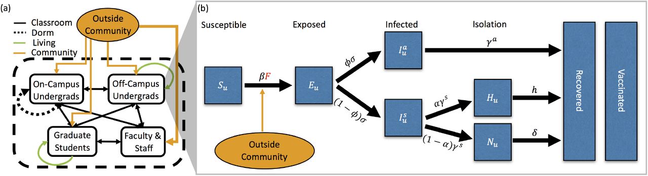
In this section, we describe the ordinary differential equation (ODE) compartment model that we have used to make most of the predictions for the university as presented to the administration during the Summer and Fall of 2020, see fig. 1(a). This SEIR model is unique as we model the four subpopulations: (1) undergraduate students living off-campus, u, (2) undergraduate students living on campus and in dorms, d, (3) graduate students, g, and (4) faculty and staff, f. Individuals are designated by both population and COVID-19 status. fig. 1(b) presents the phases of the diseases for one of the subpopulations, the undergraduate students living off campus (u).

(a) Contacts between the 4 campus populations (on-campus undergraduates (d), off-campus undergraduates (u), graduate students (g), faculty/staff (f)) and the outside community. Contacts are separated into classroom (black), dormitory (black dotted), off-campus housing (green), and the outside community (orange). Thickness of arrows corresponds to the number of contacts. (b) The stages of the COVID-19 infection, included in the ODE model, that an undergraduate living off-campus would progress through: susceptible (S), exposed (E), asymptomatically infected (Ia) or symptomatically infected (Is), if symptomatically infected individuals can choose to self-isolate (at home) (H) or not (N), and finally both asymptomatically and symptomatically infected recover (R). Note that some percentage of the population is initially vaccinated and, for simplicity, we consider them to be in the vaccinated compartment from the beginning of the simulation.
A susceptible (S) individual may become exposed (E) to SARS-CoV-2 (the virus that causes COVID-19) by coming into contact with any infected individuals (I) in any of the 4 subpopulations or the outside community (off campus). All exposed individuals become infected, either asymptomatically (Ia) or symptomatically (Is). Symptomatic individuals may choose to self-isolate and/or report to health services for testing (H) or not (N). Finally, as we do not model disease mortality, all infected individuals eventually recover (R). Vaccinated individuals (V) are unable to contract the virus nor pass it to susceptible individuals. We do not dynamically model the vaccinated population, rather they represent a subset of each subpopulation, which are removed from the susceptible class and put into the vaccinated class at the start of the simulations. fig. 11 in the Appendix shows all the subpopulations and all the phases of the disease for each subpopulation.
The equations for each stage of the infection corresponding to this subpopulation are


 where the Force of Infection, F, includes the contacts between this subpopulation and all subpopulations and the outside community,
 where cij = C(i, j) denotes the (i, j)-th entry of the contact matrix C. The equations for all stages for all subpopulations are given in Appendix A.
The model has two types of parameters: (i) parameters related to COVID-19 epidemiology and (ii) parameters related to contact patterns between the 4 subpopulations and the outside community (the matrix C, described in table 2). Details of the first type of parameters are given in table 1. Details of contacts are given below in section 3. The critical term in our model is the Force of Infection, defined in eq. (2), which governs the spread of COVID-19 and is impacted by interventions such as mask-use, quarantine of infected individuals, and changes in social connectivity, including class-size and housing caps through both types of parameters. We account for the effect of masks with our mask efficiency parameter which, when used in classrooms, reduced the transmission probability β by a factor (1 −m). We account for a quarantine period with α to represent the probability that a symptomatic individual chose to self isolate. Finally, changes in social connectivity - such as changes in class-sizes, are implemented by modifying the appropriate contact matrix.
The contact matrix C represents the total contacts within and between subpopulations, broken down by classes, living situations, outside community engagement, and social interactions.
Because our goal is to consider sensitivity of COVID-19 dynamics to NPIs in the context of a vaccinated campus population, we consider two simplifying assumptions allowing us to include vaccinated individuals in each of our campus subpopulations. First, our goal is to model COVID-19 in the context of a university environment. As such, we followed the requirements of the University of California, which requires vaccination before the semester begins and did not consider an on-going vaccination program. Second, we assume perfect vaccine efficiency by including all vaccinated individuals in the recovered category at time t = 0.
2.2 Infection Doubling Time
We are interested in analyzing the effect of intervention strategies and vaccination on the resulting dynamics of COVID-19 infections on our campus. In our work, the infection doubling time, tΔ, is the characteristic number of days for the cumulative number of COVID-19 infections to double, C(ti+1) = 2C(ti), where ti+1 = ti + tΔ for i ≥0 and t0 is a point in time at the beginning of the semester, see fig. 2. This quantity is a characteristic of the disease dynamics during the early stages of disease spread (beginning of the semester), when the number of on-campus infections remains low and the susceptible population remains large [27]. This characteristic captures the start of a semester when students that are allowed back to campus have been tested for COVID-19 (large susceptible population), and the probability that an infected student returns to campus is low. Infection control measures aimed at “flattening the curve” means increasing the case doubling time [28]. In this work we use the epidemic doubling time as a measure of epidemic dynamics to asses which intervention strategies are associated with increased variance in the doubling time.

The figure illustrates the doubling of the cumulative number of infections with respect to the infection doubling time (tΔ). Here, C(ti) is the number of infections at a time ti since the beginning of the semester.
During this initial period of disease spread, at the beginning a semester, we observe an exponential growth phase in the number of infections (fig. 2). If the number of infections is growing at a rate r, the disease doubling time is given by tΔ = log(2)/r [29]. In this early stage of approximately exponential growth in the number of cumulative case, C(t), where C′(t) ≈ rC(t), we can estimate r by using cumulative cases at two points in time C(t1) and C(t2), where r = log (C(t1)/C(t2)) /(t1 − t2) and t1 > t2. Then, the doubling time is
 In this work, we use the average doubling time computed over consecutive days in the first month (four weeks) of the semester (See fig. 2).
2.3 Global Sensitivity Analysis
In this work we are interested in understanding how particular COVID-19 SEIR epidemic model factors θ = (θ1, θ2, …, θk), table 1, affect a model response Y (the cumulative number of infections, C(t), and the disease doubling time, tΔ). We perform a variance based global sensitivity analysis on these epidemic dynamics with the Sobol method [30, 31, 32], an approach to decompose the response variance by single and combined factor interactions
 Under this decomposition, the proportion of variance from a single factor, the first-order index, can be written as
 where E is expectation, Var is the variance, θi is the ith model factor, and θ∼i indicates varying all factors except θi. In our work, a second quantity of interest is the total-order index, or total-effect index [33], which in addition to the first-order index information, accounts for the additional contribution of a factor to the model variance from interaction effects with other model factors
 It follows that
  , and that a total-order index value of zero indicates that the model factor is non-influential. In our analysis we estimate the first-order and total-order indices through numerical model solutions generated by sampling from the input factor parameter space following [30].
3 Data and Contacts
While the results we present here are specific to UC Merced, we note that any interested bubble-like communities could calculate their contacts as we outline below and use the model to make predictions. For example, our model can be applied to skilled nursing facilities (where in-patients would be equivalent to ‘on-campus students’, out-patients would represent ‘off campus students’, doctors might correspond to ‘faculty/staff’, and therapists/nurses might translate to ‘graduate students’. ‘Classes’ in this case would be face-to-face treatments). UC Merced is a public land-grant university set in a rural community. In these calculations, there were 8,334 undergraduate students, of whom 2,885 live on campus and 5,449 live off-campus. There were 723 graduate students and 424 faculty and staff. Lecturers and postdocs are considered part of the faculty/staff population. We expect our results would hold for similarly-sized campuses with similar class structures. Although we are able to get exact data from the registrar, we provide a template that can be used to estimate the contacts between different subpopulations.
For our model to be accurate, it is necessary to be able to estimate the number of contacts each of the subpopulations (off-campus undergraduates, on-campus undergraduates, graduate students, and faculty/staff) has with one another. We assume that the majority of these contacts come from inclass instruction, living/dorm situations, contact with the outside community, and unscheduled social interactions. For simplicity this information is displayed as a contact matrix in table 2. We do not dynamically model the outside community and so the contact matrix is of size 4 ×5, since the interactions of campus population do not influence the outside community.
In the following subsections, we will discuss how the contact matrix is filled using in-class instruction, living situation, outside community interaction, and unscheduled social interaction information. Each of these sections fill out a different part of the contact matrix, as described in table 2.
3.1 In-Class Instruction
The majority of interactions in our model are derived from classroom instruction. We assume that lectures are comprised of 3 hours per week, while discussion sections meet for one hour per week. When a class is listed as a lab, we assume that it meets for 2.5 hours per week. Further, we assume that faculty and staff only interact with each other during faculty meetings. In particular, we assume a faculty meeting occurs once every other week for an hour. The ‘average’ department size was calculated using information from UC Merced School of Natural Sciences, and was roughly 17.5 faculty per department.
We display the relevant information for calculating classroom contacts in table 3. Classroom contacts only influence the campus subpopulations (not the outside community) and thus the fifth column (not displayed in table 3) consists of all zeros. We note that in table 3, the classes graduate students teach as graduate assistants may be labs or discussion sections, the classes faculty & staff teach may be lectures, labs, or discussion sections.
A schematic for calculating the contact matrix due to teaching and class interactions at a university. Since classes only occur for the university community, this represents a 4 × 4 submatrix of Table 2.
3.1.1 Network Analysis
Although we use the contact matrices to model the connectivity of the campus, we can also use network analysis since we have access to individual-level data. In particular, we can build a network graph of every individual on campus and their connectivity to each other via classes only. From this network, we can determine characteristics of those individuals that have the highest rates of contact. These network analyses are presented in Appendix B.
To build the weighted undirected graph, we consider each individual affiliated with the university as a separate node. Edges are formed between two nodes if those two individuals share a class (either as students or as student/instructor). For each additional class individuals share, the edge weight is increased by one. Of course, the graph changes depending on whether all classes meet in person, or whether there is a class capacity. fig. 13a displays the resulting network for a full campus in which all classes meet in person. The network is colored by sub-population (reddish purple corresponds to oncampus undergraduates, yellow represents off-campus undergraduates, sky blue for graduate students, and vermilion for faculty), the size of each node represents the weighted degree, and the edge thickness reflects weights. It is apparent that under normal conditions most of the campus is connected with one another. However, as seen in fig. 13d, when classes with more than 25 students enrolled do not meet in person, much of the network becomes disconnected, i.e., having no contact with any other individuals. With a resulting graph for the no intervention strategy that has over 9000 nodes and 1.5 million unique edges, it becomes necessary to use metrics to analyze exactly how the campus is connected. We report a histogram distribution of the weighted degree, a measurement calculating how many edges each node has. Histogram representations of the degree are displayed in fig. 12, where the upper left panel contains no interventions and the lower right panel assumes classes that are larger than 25 students do not meet in person. It is clear that capping in-person classes has a dramatic effect on the weighted degree, reducing maximal degree from 1415 to 216. In fact, edges are reduced to ≈0.13 million. Further, approximately 17% of campus individuals have 0 classroom contacts (no edges) when implementing a class cap strategy.
We can gather information about possible ‘super-spreaders’ by examining the individuals that have the highest degrees. Under the assumption of no interventions, it is clear the individuals with the highest degree are most often undergraduate students taking many introductory classes. For example, the individuals with the top 3 degree scores were all undergraduate students taking 4-5 lower level introductory class (all living off-campus). When class caps are implemented, the structure of those with the highest interactions changes. Of the top 3 degree scores when imposing a class cap of 25, we have one lecturer teaching multiple labs and two graduate students that are taking a full load of classes and also teaching discussion sections and labs. This highlights how important it is to incorporate these sub-populations, who may serve as a vector for disease transmission, in our model.
3.2 Living Situations
In addition to classroom contacts, most members of the community will also interact with other individuals based on their living situation. We assume that the living contacts are based on living situation only. Therefore, there is no mixing between subpopulations in our model. For example, oncampus undergraduate students do not live with off-campus undergraduate students and vice versa. This means that in our contact matrix (table 2), living contacts exist only on the diagonals.
We assume that on-campus undergraduate students have contacts for approximately 20 hours/day with their direct roommate. To simulate the effects of encountering other individuals in their dorm, we assume that on-campus undergraduate students have 2 hours of contact per day multiplied by the average number of beds/bathroom. For example, if there are roughly 4 students per bathroom, they would experience 8 hours of additional contact per day.
The off-campus undergraduates are assumed to live with, on average, 3 off-campus undergraduate housemates. Since their living situation is likely larger than a dorm room, we assume less contact, at 10 hours/day contact with each roommate. Graduate students have a similar situation, except that we assume they live with 1.5 other graduate student housemates. Similarly we assume 10 hours of contact per day with each roommate for each graduate student. We assume that faculty and staff to do not live with other faculty and staff.
3.3 Contact with Outside Community
One of the most important aspects about a bubble-like community, from an infectious disease perspective, is that some key individuals have contact with the “outside community”. This is often overlooked in mathematical models, partly because the populations that interact with the outside world tend to be outnumbered by those contained fully in the bubble. However, these outside contacts cannot be ignored because they represent the potential for infection to infiltrate the “closed” community. These contacts are present in the fifth column of the contact matrix displayed in table 2.
There are varying levels of contact with the surrounding community depending on which subpopulation a person is part of. We assume that there is little contact with the outside world if you live on campus (1 hour of contact/day). For off-campus undergraduate students and graduate students, the number of contacts is higher due to increased shopping, transportation, etc. at 5 hours of contact/day. We assume that faculty and staff have the highest amount of contact with the outside community since many faculty live with families that are not affiliated with the university (15 hours of contact/day). However, as these numbers are not directly produced from known data, we also include a parameter c, that is a multiplier in front of the community contact matrix, that we vary.
3.4 Unscheduled Social Interactions
One aspect of contact that has not yet been addressed is contact that occurs outside the classroom and living situation. In particular, we consider the effect of “unscheduled” social interaction in which members of the undergraduate student population meet for gatherings, unmasked, on a daily basis. Examples of these daily social interactions might include eating dinner with friends in the dining hall or forming an in-person study group for a course. In our contact matrix (table 2), these are included in the undergraduate student populations (both on and off campus).
We incorporate unscheduled social interactions in our model in two ways: first the daily weekday interactions described above and secondly an increase in social interaction during the weekend. To calculate the daily social interactions, we assume that all students have, on average, p hours of unscheduled social contact per day, split roughly 75% with their own sub-population (on-campus to on-campus and off-campus to off-campus) and 25% with the other undergraduate sub-population (oncampus to off-campus). For the increased social interaction over the weekend, we multiply these daily social contacts by the parameter w, to simulate going to a larger gathering. This parameter and larger number of contacts is active from 5pm Friday until 5pm Sunday.
4 Results: Global Sensitivity Analysis
We are interested in the sensitivity of the cumulative number of infections at a point in time since the semester began, C(ti), and the sensitivity of the infection doubling time, tΔ, to the model parameters. We estimated the first-order sensitivity index and the total-order effect through numerical model solutions generated by sampling from the input factor space, assuming that all parameters were uniformly distributed in their given range listed in table 1, following [30]. To adequately sample the multidimensional input factor space, we apply Latin hypercube sampling implemented in [34] and use N (k + 2) simulations where k is the number of parameters we are varying, k = 17 in this work, and N is the number of simulations for each parameter, N = 1, 200 in this work. To estimate the first-order index, eq. (3), we use the estimator presented in [30] (Table 2, row b in their work). The total-order index  is estimated with the estimator presented in [35] and in [30] (Table 2 row f in their work). All confidence intervals were computed by resampling the N (k + 2) simulations 2000 times with replacement.
4.1 Variance in Cumulative Infections and Infection Doubling Time
We first study the variance of the following model metrics: the time-varying cumulative infections, the doubling time and number of the cumulative infections at the end of the fifteen-week term. As mentioned above, we do this by employing a global sensitivity analysis approach where we vary parameters independently and uniformly over their ranges. In our analysis we consider the behavior of varying three classes of parameters: infection parameters (β, σ, φ, α), contact parameters (M, c, ω, p, m), and initial conditions ( where y ∈ {s, a} and x ∈ {d, u, g, f}). (See Table 1 for ranges and details.)
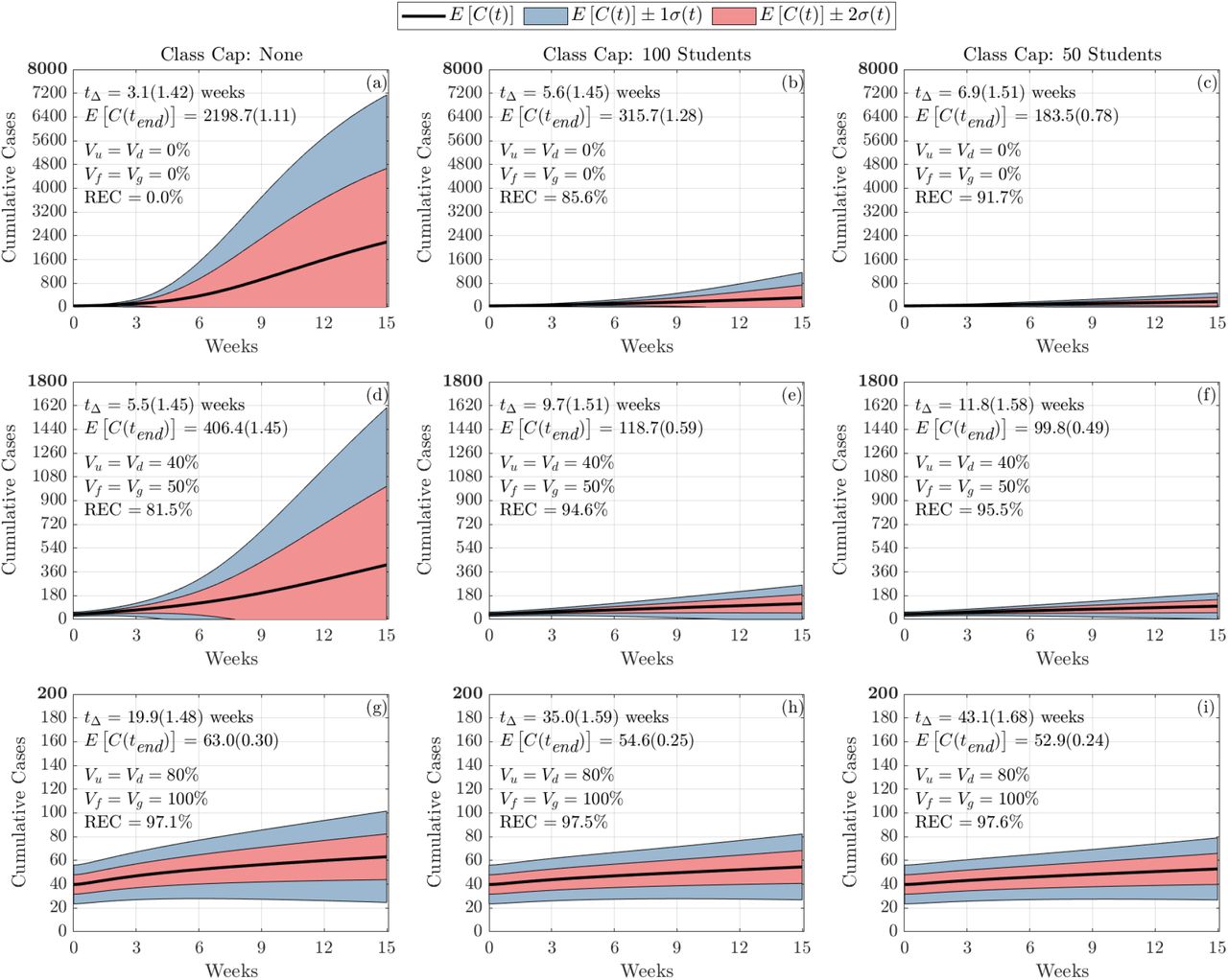
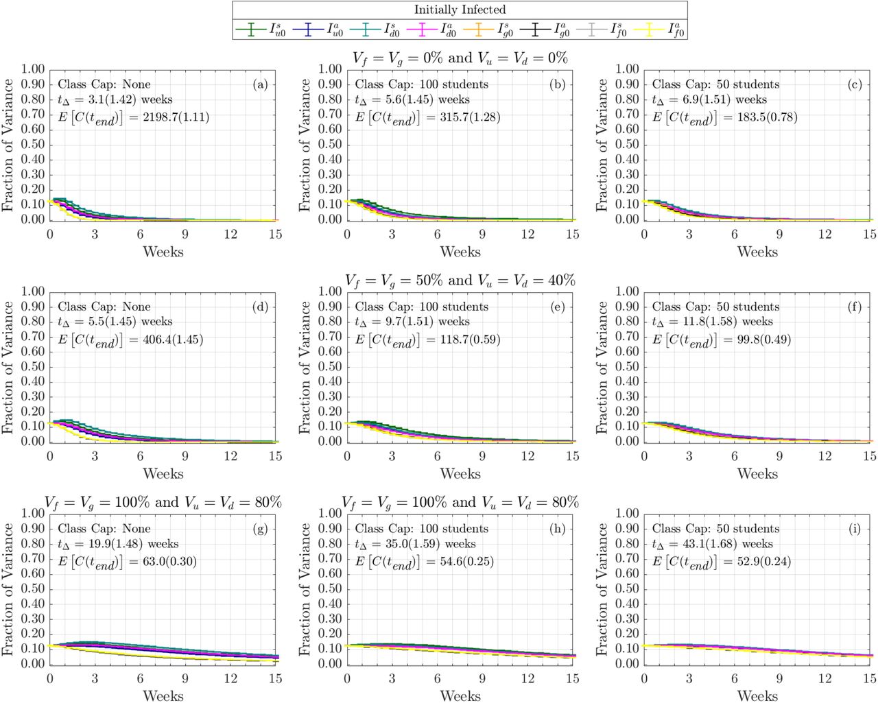
fig. 3 shows the behavior of the cumulative number of infections as a consequence of class caps (each column represents a different class cap: none, 100 students and 50 students) and vaccination status of the campus (each row). For simplicity, we assume that all undergraduates have the same vaccination fraction Vu = Vd and that graduate students and faculty have the same vaccination fraction Vf = Vg. We consider the following scenarios, Low: Vu = Vd = 0%, Vf = Vg = 0%; Medium: Vu = Vd = 40%, Vf = Vv = 50%; and High: Vu = Vd = 80%, Vf = Vg = 100%. The black line signifies the mean cumulative infections over time, while the pink and blue shadings show one and two standard deviations from the mean, respectively. The mean and standard deviations of the doubling time and total cumulative infections are reported in each subplot.

Figures show the distribution of cumulative infections over the span of a semester (15 weeks) where all students are allowed back to campus, 5449 students live off-campus and 2885 students live in the dorms, and we allow the contact, infection parameters, and initial number of infected individuals to vary (see table 1). The reduced expected cumulative infections (REC) from Fall 2019 with no vaccination and no class caps is presented in (a).
Without vaccination or class caps (fig. 3(a)), we expect nearly 2200 cases by the end of the semester. By implementing a class cap of 50 students, the expected cumulative cases drops to 184 (fig. 3(c)). On the other hand, increasing vaccination rates to 100% of faculty and graduate students and 80% for undergraduate students reduce expected cumulative cases to 63 (fig. 3(g)). When implementing both class caps and increased vaccination, we expect 53 cases by the end of the semester (fig. 3(i)). The cumulative effect of both strategies is minimal.
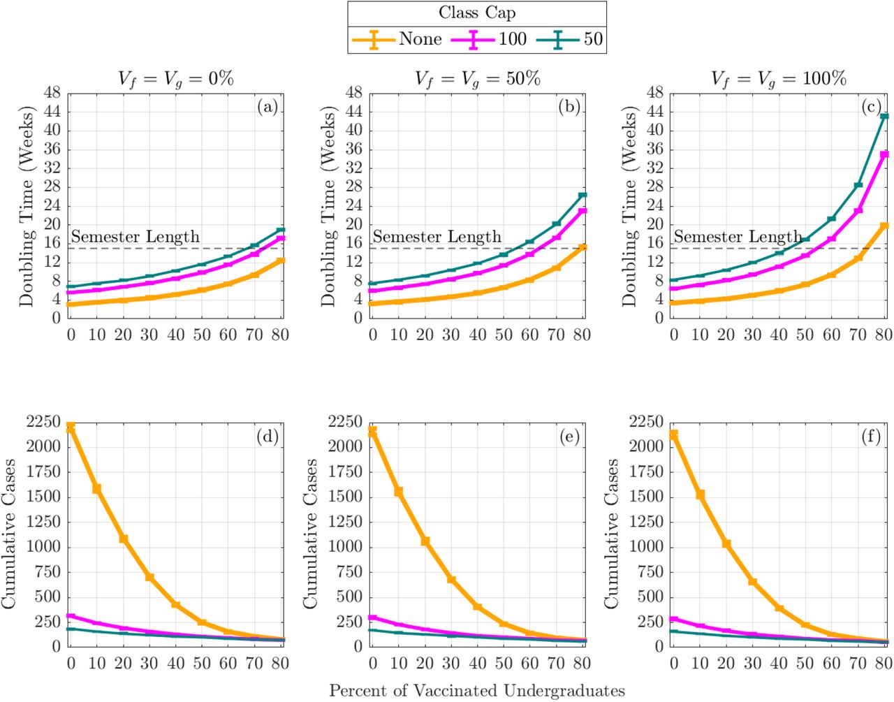
In addition to examining the cumulative number of infections, we can also investigate how vaccination and class schedule impact the doubling times of cases. fig. 4 displays the doubling time in weeks (top row) and cumulative cases at the end of the semester (bottom row) as a function of vaccinated undergraduate students, Vu = Vd. The columns represent increasing faculty and graduate student vaccination rates ranging from 0% (left), 50% (middle), and 100% (right). Within each panel, the effects of incorporating class caps are portrayed with no class cap (yellow), 100-person cap (pink), and 50-person cap (teal). As we increase undergraduate student vaccination rates, we can observe a lengthening of doubling time of the disease. Moreover, when paired with increased faculty and graduate student vaccination rates, we find that doubling times often exceed the length of the semester. At all levels of vaccination, incorporating class caps results in a modest increase in doubling time.

The expected cumulative number of infection (Cumulative Cases) by the end of the semester and the expected doubling time computed during the first four weeks of the semester. The error bars are a 95% confidence interval.
It is apparent that the non-pharmaceutical intervention of having large enrollment classes remote drastically reduces the number of cumulative cases by the end of the semester, especially when the campus population is not significantly vaccinated (fig. 4(d)-(f)). In the case when none of the population was vaccinated, by capping classes at 50 students, there is a 91.7% reduction in the expected cumulative infections by the end of the semester (fig. 3(c)). Increasing the percentage of the vaccinated population also has a large effect in reducing the cumulative cases by the end of the semester. In the case when there is no class cap, having 80% of undergraduates and 100% of faculty, staff, and graduate students vaccinated resulted in a 97.1% reduction in the expected cumulative infections by the end of the semester (fig. 3(g)).
4.2 Sobol Analysis of the Variance in Cumulative Infections and Infection Doubling Time
The first-order Sobol sensitivity index Si measures the direct effect that each parameter θi has on the variance of the model output. The total-order Sobol sensitivity index  measures the total effect (direct and through interactions with other parameters) each parameter θi has on the variance of the model output. As mentioned above, we consider the sensitivity of two model outputs: the cumulative number of infections in time and the doubling-time of the infection. We categorize the parameters for the sensitivity analysis into three groups: infection parameters (β, σ, φ, α), contact parameters (M, c, ω, p, m), and initial conditions
  . In each sensitivity analysis figure, we show 9 subfigures illustrating three class cap scenarios—no class cap (the first column), class cap with 100 students (the second column), and class cap with 50 students (the third column)—along with three vaccination scenarios—(i) 0% vaccination (the top row); (ii) 50% of faculty, 50% graduate students, and 40% of undergraduate students vaccinated (the middle row); and (iii) 100% of faculty, 100% graduate students, and 80% of undergraduate students vaccinated (the bottom row).
We note that the initial conditions do not contribute to the sensitivity of either of our metrics in a fashion that is dependent on the vaccination or non-pharmaceutical invention. As such, we include those figures in Appendix C.
4.2.1 Doubling Time
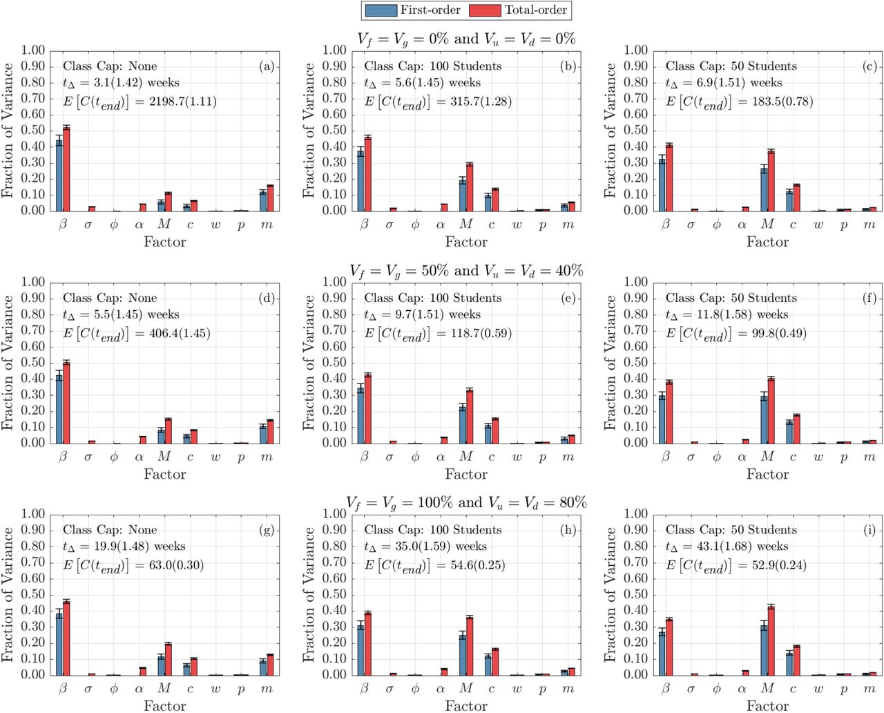
We now turn to examine the global sensitivity analysis with respect to epidemic doubling time. fig. 5 displays the global sensitivity analysis of the epidemic doubling time for the infection and contact model parameters, while fig. 14 portrays the global sensitivity analysis of the epidemic doubling time with respect to the initial conditions. First-order (blue) and total-order (red) are shown as well as the standard errors. The columns represent class caps (moving right across the columns), while the rows signify increasing levels of campus vaccination (moving down the rows). The mean and standard deviations of the doubling time and total cumulative infections are reported in each subplot.

Each column represents three class cap scenarios: none, 100 student, and 50 student caps. Each row represents one of three vaccination scenarios at the start of the semester. First row: 0% vaccination; second row: 50% of faculty, 50% graduate students, and 40% of undergraduate students vaccinated; third row: 100% of faculty, 100% graduate students, and 80% of undergraduate students vaccinated.
When examining fig. 5, we can see that with no vaccination and no class caps (fig. 5(a)), the transmission rate β is the most significant parameter. Thus, anything that can be done to lower the transmission rate, such as wearing masks or improving HVAC systems, can have a large impact on the doubling time. Other parameters that are especially sensitive are 1 − m, the reduction in transmission probability by wearing a mask, and community-related parameters M and c. M represents the percentage of infected individuals in the outside (Merced) community, while c signifies the amount we multiply the calculated contact matrices with the community. Two of the parameters, σ (representing the amount of time spend in the ‘exposed class’) and α, the probability that one self-isolates two days after symptom onset, are sensitive in total effect only. This indicates that σ or α alone do not contribute significantly to the model variance, but the interaction with other parameter(s) have a significant impact on the model variance.
As we implement the interventions, either by increasing vaccination rates (moving down the rows) or instilling class caps (moving right across the columns) we begin to see that the transmission probability, β, becomes less sensitive. On the other hand, contact with the outside community (c), and the current infection rate of the community (M) become much more important to controlling spread of the disease on campus. In fact, for some scenarios, it is clear that the infection rate of the community is more sensitive than the transmission probability. This analysis highlights the importance of including community interactions in models of bubble-like communities. Moreover, an effort to reduce transmission on campus goes hand-in-hand with increasing vaccination in the surrounding community. As we increase vaccination rates, we can see that the impact of reduction in transmission probability while wearing a mask, 1 − m, stays rather consistent in its importance. This indicates that masks are still crucial for controlling spread of disease even as vaccination rates increase. However, when decreasing the class caps, we can see that m becomes much less sensitive. Thus, NPIs, such as wearing masks and reducing contact by moving courses online, are still paramount to controlling the number of cases on campus.
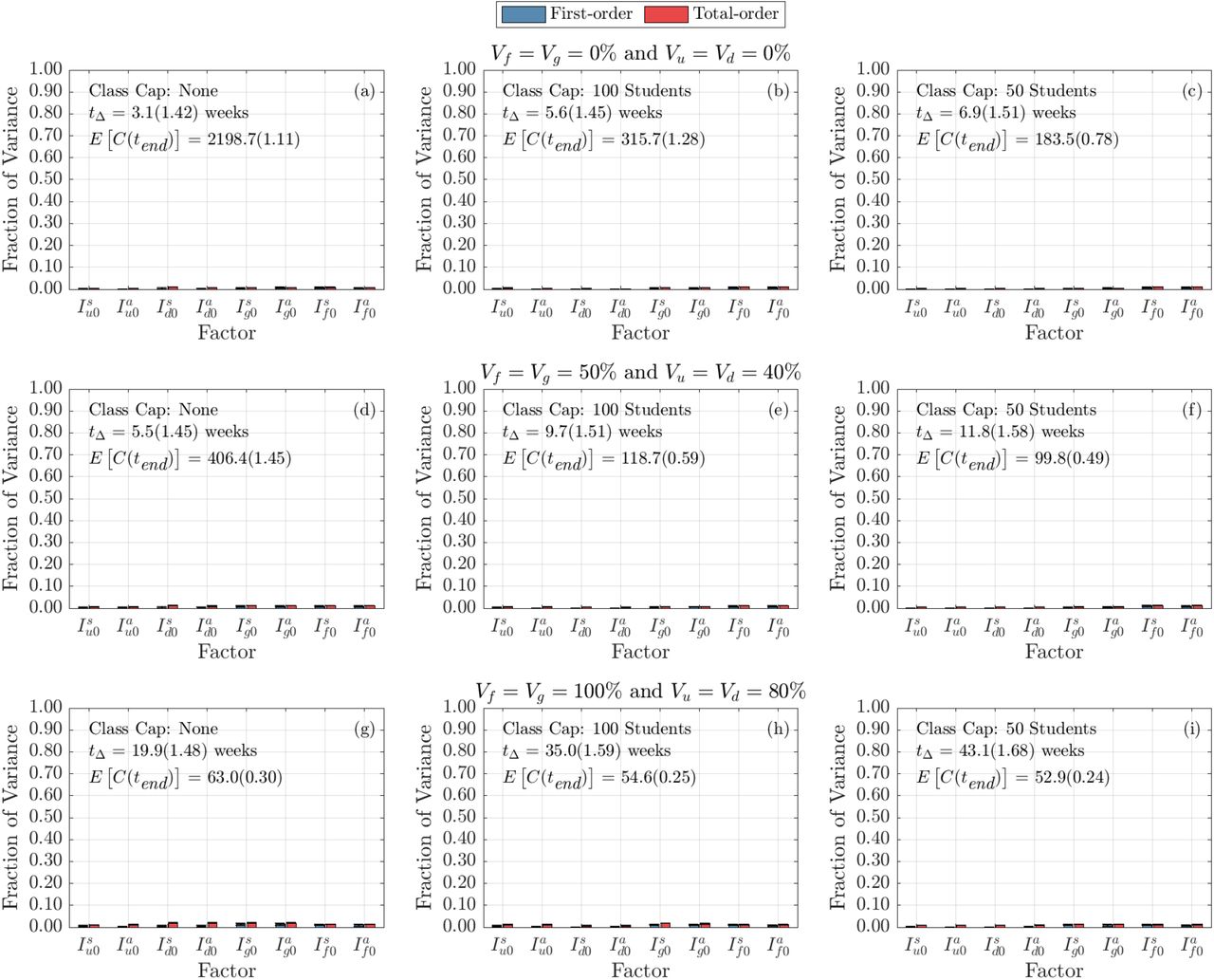
fig. 14 displays the sensitivity of doubling time for the number of initially infected individuals on campus. It is clear that the distribution and number of initially-infected individuals (undergraduate students, graduate students, and faculty and staff) do not play a large role in determining the doubling time. This is intuitive, since doubling time measures the time it takes to double the number of infections and should be the same whether we start with one infectious individual or 100 infectious individuals (see fig. 2). The interesting aspect of this analysis is that there does not appear to be a strong indication that doubling time is sensitive to whether or not those infectious individuals were asymptomatic or symptomatic. Moreover, it is similarly unimportant from which demographic group the initially-infected individuals belong to.
4.2.2 Cumulative Infections
Figure 6 displays the global sensitivity analysis for the cumulative infections at the end of the semester with respect to infection and contact parameters. As vaccination rates increase and class caps are implemented, the most sensitive parameters begin to change. Under the normal scenario, with no vaccinations and no class caps, the most important parameters are the transmission rate, β, reduction in transmission probability while wearing a mask, 1 − m, and the likelihood that a symptomatic individual decides to self-isolate, α. By incorporating class caps, the landscape of sensitivity starts to change. Self-isolation and masks become less important, while the parameters governing the outside community start to play a larger role. The probability that Merced community individuals are infectious, M, and the community contact multiplier, c, start to largely influence the cumulative number of infections. This underscores the importance of educating local communities to help reduce community spread. As vaccination increases in the absence of class caps, we see a similar shift towards community parameters being more important, however, in this scenario, mask usage remains essential towards lowering cases on campus. When both vaccination and class caps are utilized, the community parameters become more important than the transmission rate.

Each column represents three class cap scenarios: none, 100 student, and 50 student caps. Each row represents one of three vaccination scenarios at the start of the semester. First row: 0% vaccination; second row: 50% of faculty, 50% graduate students, and 40% of undergraduate students vaccinated; third row: 100% of faculty, 100% graduate students, and 80% of undergraduate students vaccinated.
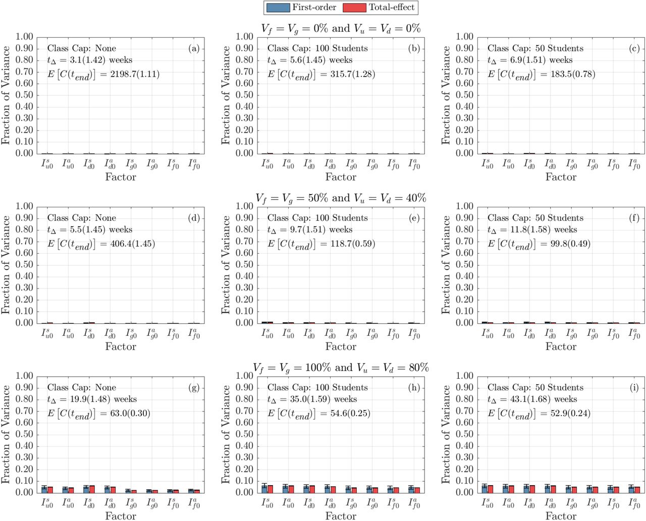
We can also examine the sensitivity of cumulative infections to the initial number of infectious individuals on campus. fig. 15 portrays this sensitivity. It is apparent that under no interventions, the initial number of infectious individuals has little effect on the spread of the virus. Similarly, when incorporating class caps, the initial conditions are insensitive. However, under high vaccination rates (80% undergraduate students and 100% faculty, staff, and graduate students), it is clear that the cumulative number of infections is slightly sensitive to the initially infectious individuals on campus – with slightly higher sensitivity to undergraduate student infections, both symptomatic and asymptomatic. In order to dissect the forces which contribute most strongly to the cumulative infections, we next consider their time-varying first and total-order Sobol indices. That is, we now look at the total contributions to the variance in cumulative infection over time. We separate the impact of infection parameters (figs. 7 and 9), contact parameters (figs. 8 and 10) and initial conditions (figs. 16 and 17). (Because the time-varying first and total order indices for initial conditions did not vary between condition, we include those figures in the Appendix C.)

Each column represents three class cap scenarios: none, 100 student, and 50 student caps. Each row represents one of three vaccination scenarios at the start of the semester. First row: 0% vaccination; second row: 50% of faculty, 50% graduate students, and 40% of undergraduate students vaccinated; third row: 100% of faculty, 100% graduate students, and 80% of undergraduate students vaccinated.

Each column represents three class cap scenarios: none, 100 student, and 50 student caps. Each row represents one of three vaccination scenarios at the start of the semester. First row: 0% vaccination; second row: 50% of faculty, 50% graduate students, and 40% of undergraduate students vaccinated; third row: 100% of faculty, 100% graduate students, and 80% of undergraduate students vaccinated.

Each column represents three class cap scenarios: none, 100 student, and 50 student caps. Each row represents one of three vaccination scenarios at the start of the semester. First row: 0% vaccination; second row: 50% of faculty, 50% graduate students, and 40% of undergraduate students vaccinated; third row: 100% of faculty, 100% graduate students, and 80% of undergraduate students vaccinated.

Each column represents three class cap scenarios: none, 100 student, and 50 student caps. Each row represents one of three vaccination scenarios at the start of the semester. First row: 0% vaccination; second row: 50% of faculty, 50% graduate students, and 40% of undergraduate students vaccinated; third row: 100% of faculty, 100% graduate students, and 80% of undergraduate students vaccinated.
First, let’s consider the time varying impact of infection parameters on the cumulative infections. As shown in fig. 7, regardless of the vaccination status or class cap scenario, the strongest contributor at all times comes from β. This is consistent with the results from fig. 6. However, we now see that this effect increases during the early part of the academic term. In addition, we note that in all cases the contribution from α, the probability that a symptomatic individual self-isolates, also increases throughout the semester. Interestingly, while the total-order index of σ, which influences the disease duration, is not necessarily monotonic. We note that in the case with no vaccination and no course caps (fig. 7(a)), σ’s strongest contribution is present around week 4 and decreases after.
Next, we move to the role of contact parameters. In fig. 8, we note that importance of contact parameters depends not only on vaccination and class-cap scenario, but also on time. As we saw in fig. 6, without a course cap the contact parameter controlling for the impact of mask use m (recall (1 − m) ∈ [0, 0.4] is the reduction in transmission rate with mask use) is the most important. Of course, as expected, the impact of mask-use on cumulative infections deceases with vaccination status of the campus. The next two most important contact factors are M, the probability that an individual in Merced, the outside community, is infected, and c, the community contact multiplier. Again, we see a time dependency. With a modest course cap, and 0% vaccination (fig. 8(b)) we note that the total-order effect of M and c increases early in the semester, but then begins to decrease around week 6 as the mask use m increases in variance contribution eventually taking over in importance by the end of the semester. This suggests that in this simulation, infections are initially coming from off campus (importance of M and c) but are then becoming dominated by on-campus spread (importance of m). We note that at the highest levels of vaccination (fig. 8(g)-(i)), the fraction of the variance from off community contact parameters M and c continues to increase as the semester goes on. This is consistent with our earlier results, but demonstrate that these factors become increasingly dominant as the semester goes on.
Not surprisingly, the importance of initial infections decreases as the term goes on for all vaccination and class cap strategies (fig. 16). We also note that, at least for the ranges and scenarios we considered, the importance of initial infections in terms of the variation in cumulative infections is far lower than the most significant infection and contact parameters.
For non-linear models, it is not generally true that the first and total order Sobol indices are consistent. However, in this case we note that the importance of parameters (i.e., the rank of their contribution to the variance) is similar for first order and total order time varying Sobol indices (compare fig. 7 to fig. 9; fig. 8 to fig. 10 and fig. 16 to fig. 17). However, there are a few intriguing differences to point out. Most notably, the first order index for β (fig. 9(a)) may exhibit an internal peak rather than simply increase to saturation. Our interpretation again would involve a change in the dynamics from early semester to later semester. For the case with no class cap and no vaccination, the transmission rate β is the parameter that has the most significant direct effect on the output variance (fig. 9(a) and fig. 10(a)). Any intervention that can lower the transmission rate β would significantly impede the transmission. As shown in fig. 9(a), we observe that the fraction of variance due to β begins to decreases after week 3 and begins increasing again after week 6. From fig. 7(a) of the time varying total-order effect, the saturation in β is due to the increasing interaction effects of σ with the other model parameters during week 3, followed by a decrease in the interaction effects after week 6. As we decrease the class cap (fig. 9, from left column to right column), the overall magnitude of the first-order effect of β remains almost the same, but at week 15, class cap 50 corresponds to the smallest fraction of variance of β. While for other infection parameters we studied, the magnitude of the first-order effect decreases as the class cap increases.
Among the contact parameters we studied, when there is no vaccination or low to medium vaccination levels (fig. 10(a)-(f)), m (mask effect on transmission rate) has the most significant direct effect on the variance of model output when there is no class cap, but the magnitude of the direct effect of M (the percentage of individuals in the outside community are infected) and c (community contact multiplier that multiplies contacts between university population and the community) exceeds m as we decrease the class cap size, with M ‘s direct effect larger than c.
Overall, both intervention strategies (class cap and vaccination) impact the direct effect of a single parameter on the variance of the model output over time. When either or both intervention strategies are implemented on campus population, the direct effect of parameters related to the outside community warrants attention.
5 Discussion and Conclusion
In this manuscript, we introduced an ODE-based SEIR model with multiple sub-populations (undergraduate students living on-campus, undergraduate students living off-campus, graduate students, and faculty and staff) on a campus that interacts with the outside community. We discussed how to use registrar information to estimate contact hours due to classes. We examined the effects of NPIs such as social distancing in the form of transitioning large classes online and masking as well as vaccinating the campus populations. We acknowledge that there are other methods of incorporating heterogeneous interactions, such as agent-based modeling and stochastic modeling [36, 37]. Our proposed model preserves some aspect of heterogeneity while remaining open to traditional methods of analysis and being computationally inexpensive. This allowed us to obtain rapid results and provide them to administration for decision making.
We examined the sensitivity analysis of various model parameters for varying levels of vaccination rates and class caps. We discovered that, as vaccination rates increase, transmission rates become less important while mask usage and keeping rates low in the surrounding community most drastically affect the case rates on campus. This highlights the need for including the non-campus community in modeling efforts and the necessity of universities to work with their surrounding communities to help limit spread.
Many of the parameters, such as the contact matrices, were directly informed from campus data. Thus, it may be that these results may not hold for other campuses that alter from our own (e.g., no large classes, campuses that are more integrated with the surrounding community, campuses in urban settings). However, our flexible framework allows other universities to alter parameters and calculate contact matrices from their registrar data, in order to make conclusions about interventions and sensitivities for their own campuses.
The parameters that were not directly calculated from data remain a source of uncertainty in the model. Although many of the parameter values were taken from literature values, the accuracy of those estimates is unknown. Therefore, model validation with real data remains a future direction for exploration. We also plan to replace the surrounding community estimate, which is currently a constant, with dynamic data from county dashboard reports. We can also study the impact of a surge in COVID cases in the off-campus community on campus population, by introducing a pulse in the community parameter.
We note there are several limitations with the current study. In our model it is assumed that vaccination makes the recipient immune (e.g., there are no breakthrough cases). A logical future direction would include waning immunity and booster shots. Another option would be to include vaccinated sub-populations with decreased transmission rates and shorter convalescence times. As differing variants have become dominant (e.g., delta, omicron), the parameters would need to be altered to reflect increased transmission rates and, perhaps, shortened infectious duration. We also assumed 100% compliance with interventions, meaning that every member of the community wears well-fitting masks at all times when they are indoors.
Overall, our model exhibits results consistent with current public health messaging. Our model predicts that, despite increasing vaccination rates, it remains important to continue to socially distance and wear masks to reduce transmission. Whether these results will hold for more recent variants, such as delta and omicron, remains to be seen.
Data Availability
Open-source code for the global sensitivity analysis and contact matrices can be found at https://github.com/FS-CodeBase/gsa_of_covid19_transmission_on_a_university_campus.
Statements and Declarations
Code and Data Availability
Open-source code for the global sensitivity analysis and contact matrices can be found at https://github.com/FS-CodeBase/gsa_of_covid19_transmission_on_a_university_campus.
Competing Interests
The authors declare that they have no competing interests.
A Details of the ODE model
In fig. 11, we show all the subpopulations, the undergraduate students who live off campus (u), the undergraduate students who live on campus in the dorms (d), the graduate students (g), and the faculty and staff (f) as they progress through the stages of the COVID-19 infection. The corresponding equation are given in eq. (4). Note that all the populations are coupled through the Force of Infection, eq. (2) in the main text, where an individual in any subpopulation can be infected by any infected individual in the total population or through a member of the community,
 where cij = C(i, j) is the (i, j)-th entry of the contact matrix C.

All subpopulations included in the ODE model, (1) undergraduate students off-campus (u), (2) undergraduate students in dorms (d), (3) graduate students (g), and (4) faculty and staff (f) and the phases of the disease that each individual progresses through: susceptible (S), exposed (E), asymptomatically infected (Ia) or symptomatically infected (Is), if symptomatically infected individuals can choose to self-isolate (at home) (H) or not (N), and finally both asymptomatically or symptomatically infected recover (R). Note that some percentage of the population is initially vaccinated.
B University Network Visualization
University network characteristics under four interventions with different class cap size. For all four cases, the total number of nodes is 9481, with nu = 5449, nd = 2885, ng = 723, and nf = 424.

Histogram of weighted degrees for the university network under four interventions with different class cap sizes. Bin width are 50, 25, 10 and 5 for No Intervention, class cap 100, class cap 50, and class cap 25, respectively.

Visualization of university network as a weighted undirected network under four interventions with different class cap size. Edge thickness reflects weights (minimum 1 and maximum 10). Nodes were colored according to their roles (reddish purple for u, yellow for d, sky blue for g, and vermillion for f) and sized according to weighted degree (smaller nodes correspond to smaller weighted degrees). See Table 4 for the breakdown of the networks.
C Figures of Sensitivity Analysis to Initial Conditions

Each column represents three class cap scenarios: none, 100 student, and 50 student caps. Each row represents one of three vaccination scenarios at the start of the semester. First row: 0% vaccination; second row: 50% of faculty, 50% graduate students, and 40% of undergraduate students vaccinated; third row: 100% of faculty, 100% graduate students, and 80% of undergraduate students vaccinated

Each column represents three class cap scenarios: none, 100 student, and 50 student caps. Each row represents one of three vaccination scenarios at the start of the semester. First row: 0% vaccination; second row: 50% of faculty, 50% graduate students, and 40% of undergraduate students vaccinated; third row: 100% of faculty, 100% graduate students, and 80% of undergraduate students vaccinated.

Each column represents three class cap scenarios: none, 100 student, and 50 student caps. Each row represents one of three vaccination scenarios at the start of the semester. First row: 0% vaccination; second row: 50% of faculty, 50% graduate students, and 40% of undergraduate students vaccinated; third row: 100% of faculty, 100% graduate students, and 80% of undergraduate students vaccinated.

Each column represents three class cap scenarios: none, 100 student, and 50 student caps. Each row represents one of three vaccination scenarios at the start of the semester. First row: 0% vaccination; second row: 50% of faculty, 50% graduate students, and 40% of undergraduate students vaccinated; third row: 100% of faculty, 100% graduate students, and 80% of undergraduate students vaccinated.
Acknowledgments
The work presented in this manuscript is based upon work supported by the National Science Foundation (DMS–1840265 and ACI-1429783), the Joint Initiative to Support Research at the Interface of the Biological and Mathematical Sciences between the National Science Foundation Division of Mathematical Sciences (NSF-DMS) and National Institutes of Health National Institute of General Medical Sciences (NIH-NIGMS) (Grant No. R01-GM126548), and UC Merced COVID-19 Seed Grant.
We would like to acknowledge Drs. Folashade Agusto, Joan Ponce, and Omayra Ortega for detailed discussions in formulating the original version of the UC Merced model. We also acknowledge the guidance and support from Dr. Thelma Hurd, Director of Medical Education, Professor of Public Health, who was the head of UC Merced’s COVID Task Force.
References


