
Abstract
Problem definition To respond to pandemics such as COVID-19, policy makers have relied on interventions that target specific population groups or activities. Since targeting is potentially contentious, rigorously quantifying its benefits is critical for designing effective and equitable pandemic control policies.
Methodology/results We propose a flexible modeling framework and a set of associated algorithms that compute optimally targeted, time-dependent interventions that coordinate across two dimensions of heterogeneity: age of different groups and the specific activities that individuals engage in during the normal course of a day. We showcase a complete implementation focused on the Île-de-France region of France, based on commonly available public data. We find that targeted policies generate substantial complementarities that lead to Pareto improvements, reducing the number of deaths and the economic losses, as well as the time in confinement for each age group. Optimized dual-targeted policies are interpretable: by fitting decision trees to our raw policy’s decisions across many problem instances, we find that a feature corresponding to the ratio of marginal economic value prorated by social contacts is highly salient in explaining the confinements that any group - activity pair experiences. We also quantify the impact of fairness requirements that explicitly limit the differential treatment of distinct groups, and find that satisfactory trade-offs are achievable through limited targeting.
Implications Given that some amount of targeting of activities and age groups is already in place in real-world pandemic responses, our framework highlights the significant benefits in explicitly and transparently modelling targeting and identifying the interventions that rigorously optimize overall societal welfare.
1. Introduction
The COVID-19 pandemic has forced policy makers worldwide to rely on a range of large-scale population confinement measures in an effort to contain disease spread. In determining these measures, a key recognition has been that substantial differences exist in the health and economic impact produced by different individuals engaged in distinct activities. Targeting confinements to account for such heterogeneity could be an important lever to mitigate a pandemic’s impact, but could also lead to potentially contentious and discriminatory measures. This work is aimed at developing a rigorous framework to quantify the benefits and downsides of such targeted interventions in pandemic management, and applying it to the COVID-19 pandemic as a real-world case study.
Targeting has been implemented in several different ways during the COVID-19 pandemic. One real-world contentious example has been to differentiate confinements based on age groups, e.g., sheltering older individuals who might face higher health risks if infected, or restricting younger groups who might create higher infection risks. Such measures have been implemented in several settings – e.g., with stricter confinements applied to older groups in Finland (Tiirinki et al. 2020), Ireland (Harrison 2020), Israel (Magid 2020) and Moscow (Foy 2020), or curfews applied to children and youth in Bosnia and Herzegovina (Reuters Staff 2020) and Turkey (Kanbur and Ankgül 2020) – but some of the measures were deemed ageist and unconstitutional and were eventually overturned (Magid 2020, Reuters Staff 2020).
A different example of targeting extensively employed in practice has been to tailor confinements to specific activities conducted during a typical day. This has been driven by the recognition that different activities (or more specifically, population interactions in locations of certain activities) such as work, schooling, transport or leisure can result in significantly different patterns of social contacts and new infections. This heterogeneity has been recognized in numerous implementations that differentially confine activities through restrictions of varying degrees on schools, workplaces, recreation venues, retail spaces, etc. Additionally, some practical implementations even differentiated based on both age groups and activities, e.g., by setting aside dedicated hours when only the senior population was allowed to shop at supermarkets (Aguilera 2020), or by restricting only higher age groups from in-person work activities (Magid 2020).
As these examples suggest, targeted interventions have merits but also pose potentially significant downsides. On the one hand, targeting can generate improvements in both health and economic outcomes, giving policy makers an improved lever when navigating difficult trade-offs. Additionally, explicitly considering multiple dimensions of targeting simultaneously – such as activities and age groups – could overturn some of the prevailing insight that specific age groups should uniformly face stricter confinements. However, such granular policies are more difficult to implement, and could lead to discriminatory and potentially unfair measures.
Given that some amount of targeting is already in place in existing real-world policy implementations, it is critical to transparently model and quantify its benefits and downsides. This gives rise to several natural research questions: How large are the health and economic benefits of interventions that can engage in progressively finer targeting? Does finer targeting lead to significant synergies, and is there an interpretable mechanism through which this happens? What is the relationship between the effectiveness and the level of targeting allowed across distinct groups?
We develop a rigorous framework and a set of associated algorithms that allow addressing these questions in concrete, real-world settings. Although the framework is flexible and allows embedding different interventions, we focus on dual-targeted confinements, that is, confinements that can target age groups and activities, as these have been the most prevalent forms of targeting seen in practice.
1.1. Contributions
Our framework overcomes two practical challenges. First, a rigorous quantification of the value of targeting must be grounded in formal optimization. To that end, we embed an optimization framework within a traditional SEIR epidemiological model that differentiates policies based on both population groups and activities, and balances the lost economic value with the cost of deaths. Since embedding complex controls into the highly non-linear, non-convex, SEIR epidemic model renders exact optimization methods not applicable, we focus on designing an algorithm that can tractably produce approximate solutions. The algorithm is a linearization and optimization procedure that we call Re-Optimization with Linearized Dynamics (ROLD), and that is inspired by model predictive control (Bemporad 2006, Camacho and Alba 2013) and trust region methods (Yuan 2015). ROLD sidesteps the lack of convexity in the original problem by repeatedly solving optimization problems that rely on a linearized approximation of the SEIR dynamical system, where each optimization problem is reduced to a linear program.
The second contribution of our paper is a real-life implementation of the aforementioned framework, which overcomes the data availability challenge associated with calibrating a finely targeted model like ours. Our calibration leverages publicly available data on (i) real-time hospitalization, (ii) community mobility, (iii) social contacts, and (iv) socio-economic measures collected during the COVID-19 pandemic in Île-de-France, a region of France encompassing Paris with a population of approximately 12 million. Our implementation combines a complex, multi-group epidemiological model with an economic model that allows quantifying trade-offs between economic activity and epidemiological impact via the ROLD algorithm.
We next leverage the framework to address the core research questions that we posed earlier. We calibrate our optimization model up to October 21, 2020, and then apply our optimization framework to derive optimal intervention policies for subsequent horizons of 90 and 360 days. We draw the following conclusions from these experiments:
Dual targeting leads to significant Pareto improvements. Specifically, the optimal ROLD policy that differentially targets both on age groups and activities Pareto dominates the optimal ROLD policies that can only target on age groups, activities, or neither, i.e., it leads to lower economic costs without increasing the number of pandemic deaths. The gains from targeting are also super-additive: targeting on both dimensions gains more than the sum of gains from unilateral targeting. In addition, age group and activity targeted ROLD Pareto-dominates a number of benchmark policies resembling those implemented in practice during COVID-19. Finally, although not an explicit objective of the optimization, the dual-targeted ROLD policy generally results in a reduction in confinements for all population groups, relative to less fine-grained policies.
Optimized dual-targeted policies have an interpretable structure, imposing less confinement on group-activity pairs that generate a relatively high economic value prorated by activity-specific social contacts. This allows ROLD to create complementary confinement schedules for different groups that reduce both the number of deaths and economic losses, with the important added benefit that they do not require completely confining any age group. To rigorously explore the interpretability of the policies produced by ROLD, we generate a training dataset by running it on an ensemble of instances, and then use CART to train trees that predict its decisions based on simple, transparent features. The resulting trees fit well and reveal that ROLD’s targeting mechanism is interpretable. The key feature that explains how the targeting is done is the “econ-to-contacts-ratio”, i.e., the ratio of marginal economic value to total contacts generated for a given (group, activity) pair; this provides policy makers with a transparent metric to explain ROLD’s decisions.
Since targeted policies could lead to increased disparities in the confinements of distinct groups and thus be perceived as unfair, we incorporate fairness considerations into our framework through “limited disparity” constraints that restrict the allowed difference in confinements faced by distinct groups, and we quantify their impact on efficiency (measured in terms of health and economic costs). While the experiments suggest that the cost of limited disparity may be high, satisfactory intermediate trade-offs may be achievable through limited targeting.
2. Literature Review
The literature on pandemic response, particularly in the COVID-19 context, is already vast, so we focus our literature review on three key dimensions that our work most closely relates to.
Targeting
Paralleling our aforementioned real-life examples, several papers have studied targeted interventions. Kucharski et al. (2020), Prem et al. (2020), Di Domenico et al. (2020) recognize the importance of heterogeneity in the social contacts generated through activities and examine several interventions limiting them. Though some of the models here are age differentiated, targeting only happens through activities. Population group targeting, either through confinements, testing or vaccinations, has been investigated in Bastani et al. (2021), Acemoglu et al. (2020), Matrajt et al. (2020), Goldstein et al. (2021), Bertsimas et al. (2020), Favero et al. (2020), Birge et al. (2020), Chang et al. (2020), Evgeniou et al. (2020), Giordano et al. (2021). By enforcing stricter confinements for higher risk groups (e.g., older populations when considering mortality risk or younger populations when considering the risk of new infections), such targeted policies have been shown to generate potentially significant improvements in health outcomes, and even in economic value if optimally tailored (Acemoglu et al. 2020). A potential benefit of our approach is that, by exploiting complementarities between group and activity targeting, these higher risk groups may experience less confinement for the same level of aggregate deaths and economic losses.
Optimization of interventions
Our proposed optimization algorithm differs in several ways from existing approaches to assessing interventions via SEIR epidemiological models. A number of papers simulate a small number of candidate interventions, e.g. full lockdown versus school-only lockdown (Kucharski et al. 2020, Prem et al. 2020, Di Domenico et al. 2020, El Housni et al. 2020, Favero et al. 2020), restrict the candidates to a simple parametric class for which exhaustive search is computationally feasible (e.g., trigger policies based on hospital admissions as in Duque et al. 2020 or confirmed cases as Ahn et al. 2021), or use global optimization methods such as simulated annealing (Dutta et al. 2021). When considering a more complex policy space like in our targeting model, such approaches can lead to significantly sub-optimal results and misleading conclusions. Another stream borrows from the optimal control literature to design non-targeted control policies for single-group and single-activity SEIR dynamics (Bose et al. 2021, Pataro et al. 2021, Morris et al. 2021). Although optimization-based, the models there are simpler than our own and do not capture targeting. Birge et al. (2020) use formal optimization for location-based targeting, but in a one-shot model that does not differentiate age groups or activities and does not account for time in the calculation of health or economic impact. The paper that is most related to ours is Bertsimas et al. (2020), which also proposes a multi-group SEIR formulation, in conjunction with an iterative coordinate descent algorithm to optimize vaccine allocations in a differentiated fashion. Although taking different approaches to doing so, both the algorithm proposed there and the ROLD heuristic crucially depend on solving linearized versions of the true SEIR dynamics which are tractable via commercial solvers. However, the model of Bertsimas et al. (2020) focuses on vaccine allocation decisions, whereas ours captures the dynamics of differential confinements and also allows activity-based targeting.
SEIR model calibration
Our work is also related to several other papers that have estimated SEIR parameters, particularly in the COVID-19 context. A number of papers estimate SEIR epidemiological parameters stratified by age groups – we use the estimates from the Île-de-France study in Salje et al. (2020). Another stream of papers, focusing on forecasting COVID-19 spread, estimate when and how the underlying SEIR parameters evolve in response to government interventions and changes in individual behavior, such as Perakis et al. (2021), Li et al. (2021). Lastly, we relate to the literature that has used Google and other mobility data to inform COVID-19 response strategies or to estimate the realized reductions in social contacts during COVID-19 (Dutta et al. 2021, Ilin et al. 2021, Wellenius et al. 2020, Cot et al. 2021, Xiong et al. 2020), as well as the literature on social contacts estimation (Béraud et al. 2015, Prem et al. 2017).
3. Model and Optimization Problem
Our framework relies on a flexible model that captures several important real-world considerations. We extend a multi-group SEIR model to capture controls that target based on (i) age groups, and (ii) types of activities that individuals engage in. Different policy interventions can be embedded: we include time-dependent confinements as well as testing and quarantining in our study, but vaccinations can also be accommodated. The controls modulate the rate of social contacts and the economic value generated, and the objective of the control problem is to minimize a combination of health and economic losses caused by deaths, illness, and activity restrictions. The model captures important resource constraints (such as hospital, ICU, and testing capacities), and allows explicitly controlling the amount of targeting through “limited disparity” constraints that limit the difference in the extent of confinement imposed on distinct population groups.
3.1. Some Notation
We denote scalars by lower-case letters, as in v, and vectors by bold letters, as in v. We use square brackets to denote the concatenation into vectors: v := [v0, v1]. For a time series of vectors v1, …, vn, we use the notation vi:j := [vi, …, vj] to denote the concatenation of vectors vi through vj. Lastly, we use v⊤ to refer to the transpose of v.
3.2. Epidemiological Model and Controls
We rely on a modified version of the discretized SEIR (Susceptible-Exposed-Infectious-Recovered) epidemiological model (Anderson and May 1992, Prem et al. 2020, Salje et al. 2020) with multiple population groups that interact with each other. In our case study we use nine groups g ∈ 𝒢 determined by age and split in 10-year buckets, with the youngest group capturing individuals with age 0-9 and the oldest capturing individuals with age 80 or above. Time is discrete, indexed by t = 0, 1, …, T and measured in days. We assume that no infections are possible beyond time T.
Compartmental Model and States
Figure 1 represents the compartmental model and the SEIR transitions for a specific group g. For a population group g in time period t, the compartmental model includes states Sg(t) (susceptible to be infected), Eg(t) (exposed but not yet infectious), Ig(t) (infectious but not confirmed through testing and thus not quarantined),  (infectious and confirmed through testing and thus quarantined; this state is further subdivided into
  for j ∈ {a, ps, ms, ss} to model different degrees of severity of symptoms: asymptomatic, paucisymptomatic, with mild symptoms, or with severe symptoms; we assume that an infectious individual in group g will exhibit symptoms of degree j with probability pj,g), Rg(t) (recovered but not confirmed as having had the virus),
  (recovered and confirmed as having had the virus), and Dg(t) (deceased). Individuals with severe symptoms will need hospitalization, either in general hospital wards (Hg(t)) or in intensive care units (ICUg(t)). All the states represent the number of individuals in a compartment of the model in the beginning of the time period.

Susceptible individuals get infected and transition to the exposed state at a rate determined by the number of social contacts and the transmission rate β(t). Exposed individuals transition to the infectious state at a rate σ and infectious individuals transition out of the infectious state at a rate µ. An infectious individual will need to be hospitalized in general hospital wards or ICU with probability  and
and  , respectively, where
  . On average, patients who are treated in general hospital wards (ICU) spend
  days in the hospital (ICU). An infectious individual with severe symptoms in group g will decease (recover) with probability
  .
.
We keep track of all living individuals in group g who are not confirmed to have had the disease Ng(t) := Sg(t) + Eg(t) + Ig(t) + Rg(t), and let Xt = Sg(t), Ig(t), …, Dg(t)] g∈𝒢 denote the full state of the system (across groups) at time 0≤ t≤ T. We denote the number of compartments by |𝒳|, so the dimension of Xt is |𝒢||𝒳| ×1.
Controls
Individuals interact in activities belonging to the set 𝒜 = {work, transport, leisure, school, home, other }. These interactions generate social contacts that drive the rate of new infections.
We control the SEIR dynamics by adjusting the confinement intensity in each group-activity pair over time: we let  denote the activity level allowed for group g and activity a at time t, expressed as a fraction of the activity level under a normal course of life (i.e., no confinement). In our study we take
  , meaning that the number of social contacts at home is unchanged irrespective of confinement policy.1 We denote the vector of all activity levels for group g at t by
  , and we also refer to lg(t) as confinement decisions when no confusion can arise.
We propose a parametric model to map activity levels to social contacts. We use cg,h(lg, lh) to denote the mean number of total daily contacts between an individual in group g and individuals in group h across all activities when their activity levels are lg, lh, respectively. Varying the activity levels changes the social contacts according to
 where
where  denote the mean number of daily contacts in activity a under normal course (i.e., without confinement), and α1, α2 ∈ ℝ are parameters. This parametrization is similar to a Cobb-Douglas production function (Mas-Colell et al. 1995), using the confinement patterns as inputs, and the number of social contacts as output. We retrieve values for
  from the data tool of Wille et al. (2020), which is based on the French social contact survey data in Béraud et al. (2015), and we estimate α1, α2 from health outcome data (French Government 2020) and Google mobility data (Google 2020), as described in Section EC.4.2.
Besides confinements, we also model targeted viral testing decisions, which capture how much of a finite capacity of tests to allocate to each age group. We model random mass testing, where a test detects an infectious individual with probability equal to the fraction of infectious individuals in the group’s population. Infected individuals in group g who are detected are placed in the quarantined SEIR state  , where they can no longer infect others. We use
  to denote the number of viral tests allocated to group g in period t. The testing decisions for the policy maker are then
  . Figure 1 represents the flows from one compartment to the other resulting from testing, for a specific group g.
Let
 denote the vector of all decisions at time t∈ {0, 1, …, T −1 }, i.e., the confinement and viral testing decisions for all the groups. We denote the number of different decisions for a given group at a given time by |𝒰|. Then the dimension of ut is |𝒢||𝒰| × 1.
3.3. Resources and Constraints
We use KH(t) (KICU(t)) to denote the capacity of beds in the general hospital wards (in the ICU) on day t. When the patient inflow into the hospital or the ICU exceeds the remaining number of available beds, then the policy maker needs to decide how many patients to turn away from each group. Although in principle our framework allows optimizing over such decisions, we choose to not consider this dimension of targeting because it can be extremely contentious in practice. Instead, we implement a proportional rule that allocates any remaining hospital and ICU capacity among patients from all age groups proportionally to the number of cases requiring admission from each group. More formally, with  and
and  denoting the number of patients from age group g who are denied admission to general hospital wards and ICU, respectively, in period t, the proportional rule is:

 where
where  and
and  denote the inflow of patients from group g into the hospital and ICU in period t, respectively. We assume that all patients that are denied admission die immediately.
We further assume a given capacity for viral tests each day, which we denote by KVtest(t) on day t. We assume that viral tests used to test individuals with severe symptoms that enter the ICU or hospital, as well as viral tests that test hospitalized individuals to confirm they have recovered, come from a different pool of tests and do not consume the capacity for viral testing in the non-hospitalized population.
We can now write a complete set of discrete dynamical equations for the controlled SEIR model ((EC.1)-(EC.11) in Appendix EC.1) and summarize these using the function
 where ΔXt := Xt+1 − Xt. Additionally, we can also write the following constraints for the optimization problem:


 We denote by 𝒞 (Xt) the feasible set described by (5)-(9) for the vector of decisions ut at time t.
3.4. Objective
Our objective captures two criteria. The first quantifies the total deaths directly attributable to the pandemic, which we denote by Total Deaths(u0:T −1) := ∑g∈𝒢 Dg(T) to reflect the dependency on the specific policy u0:T −1 followed.
The second criterion captures the economic losses due to the pandemic, denoted by Economic Loss(u0:T −1). These stem from three sources: (a) lost productivity due to confinement, (b) lost productivity during the pandemic due to individuals being quarantined, hospitalized, or deceased, and (c) lost value after the pandemic due to deaths (as deceased individuals no longer produce economic output even after the pandemic ends).
To model (a), we assign a daily economic value vg(l) to each individual in group g that depends on the activity levels l := [lg]g∈𝒢 across all groups and activities. For the working age groups, vg(l) comes from wages from employment and is a linear function of group g’s activity level in work  and of the average activity levels in leisure, other and transport for the entire population (equally weighted). This reflects that the value generated in some industries, like retail, is impacted by confinements across all these three activities. For the school age groups, vg(l) captures future wages from employment due to schooling and depends only on the group’s activity level in school
  . For (b), we assume that an individual who is in quarantine, hospitalized, or deceased, generates no economic value. For (c), we determine the wages that a deceased individual would have earned based on their current age until retirement age under the prevailing wage curve, and denote the resulting amount of lost wages with
  .
.
The overall economic loss is the difference between the economic value that would have been generated during the time of the pandemic under a “no pandemic” scenario, denoted by V, and the value generated during the pandemic, plus the future economic output lost due to deaths.
 All the details of the economic modelling are deferred to Appendix EC.2.
To allow policy makers to weigh the importance of the two criteria, we associate a cost χ to each death, which we express in multiples of French GDP per capita. Our framework can capture a multitude of policy preferences by considering a wide range of χ values, from completely prioritizing economic losses (χ = 0) to completely prioritizing deaths (χ → ∞).
3.5. Optimization Problem
The optimization problem we solve is to find control policies (for confinement and testing) that minimize the sum of mortality and economic losses2 subject to the constraints that (i) the state trajectory follows the SEIR dynamics, and (ii) the controls and states respect the capacity and feasibility constraints discussed above. Formally, we solve:


4. Algorithm: Re-Optimization with Linearized Dynamics
Before describing our approach to solving problem (11)-(13), we first comment briefly on the challenges in solving this problem to optimality, i.e. without resorting to approximation methods. A key term in the dynamics of any SEIR-type model is the rate of new infections, which involves multiplying the current susceptible population in a given group with the infected population in another group. This introduces non-linearity in the state trajectory; for instance, our dynamic for the evolution of the susceptible population in group g from (EC.2) reads:
 It can be easily seen that expanding out Sg(t) produces a nested fraction of polynomials in all the past decisions l(τ), N Vtest(τ) for 0 ≤ τ ≤ t− 1.3 This function has no identifiable structure that would make the resulting optimization problem tractable via convex optimization. Similarly, the objective also involves products of states and controls, and suffers from the same lack of convexity.
With this in mind, we focus on developing heuristics that can tractably yield good policies, and propose an algorithm, which we call Re-Optimization with Linearized Dynamics, or ROLD, that builds a control policy by incrementally solving linear approximations of the true SEIR system.
4.1. Linearization and Optimization
The key idea is to solve the problem in a shrinking-horizon fashion, where at each time step k = 0, …, T we linearize the system dynamics and objective (over the remaining horizon), determine optimal decisions for all k, …, T, and only implement the decisions for the current time step k.
We first describe the linearization procedure. Recall that the true evolution of our dynamical system is given by (4). The typical approach in dynamical systems is to linearize the system dynamics around a particular “nominal” trajectory. More precisely, assume that at time k we have access to a nominal control sequence  and let
  denote the resulting nominal system trajectory under the true dynamic (4) and under
  . We approximate the original dynamics through a Taylor expansion around
  :
:
 where ∇XFt and ∇uFt denote the Jacobians with respect to Xt and ut, respectively. Note that these Jacobians are evaluated at points on the nominal trajectory, so (14) is indeed a linear expression of Xt and ut. By induction, every state Xt under dynamic (14) will be a linear function of uτ for τ < t, and all the constraints will also depend linearly on the decisions.
In a similar fashion, we also linearize the objective (11). Since vg(l(t)) is linear in ut for all t = 0, …, T − 1, the objective contains bilinear terms and can be written compactly as:
 for some matrix M with dimensions |𝒢||𝒰| × |𝒢||𝒳|, and vectors γ and η of dimensions |𝒢||𝒳| ×1 (detailed expressions are available in Appendix EC.3). By linearizing this using a Taylor approximation, we consider the following objective instead:
 which depends linearly on all the decisions u0,…, uT −1.
Linearization-optimization procedure
We use the following heuristic to obtain an approximate control at time k, for k = 0,…, T − 1:
Given the current state Xk and a nominal control sequence
 for all remaining periods, calculate a nominal system trajectory under the true dynamic in (4). (The nominal control sequence is set to a solution obtained by a gradient descent method at k = 0, and to the algorithm’s own output from period k− 1 for periods k > 0, per Step 4 below.)
Use (14) to approximate the state dynamic around the nominal trajectory
and use (16) to approximate the objective-to-go function over the remaining periods t ∈ {k, …, T }.Solve the linear program to obtain decision variables
that maximize the linearized objective-to-go subject to all the relevant linearized constraints.Set the nominal control sequence for the next time step as
.Update the states using the optimal control
and the true dynamic in (4), i.e..


The linearization-optimization procedure described above is run for all periods k = 0, …, T − 1 sequentially to output a full control policy .
.
Trust region implementation
In our experiments, we have found that the linearized model described in (14) may diverge significantly from the real dynamical system when the optimized controls  determined in Step 3 diverge sufficiently from the nominal controls
  considered in the linearization in Step 2. This can lead to a large sensitivity in performance to the initialization used in the very first step; for example, if the Taylor approximation were constructed around a policy of full confinement, the linearized model could systematically underestimate the number of infections and deaths created when considering more relaxed confinements.
We overcome this by employing an iterative procedure inspired by a trust region optimization method. The key idea is to avoid the large approximation errors by running the linearization-optimization procedure iteratively within each time step k, with each iteration only being allowed to take a small step towards the optimum within a trust region of an ϵ-ball around the nominal control sequence  , and the updated optimized control sequence of each iteration being used as a nominal sequence for the next iteration. This leads to a procedure that is much more robust to the initial guess of control sequence, albeit at the expense of increased computation time.
Further algorithmic details for ROLD are provided in Appendix EC.3.
5. Île-de-France Model Parametrization, Calibration and Experimental Setup
In this section we summarize our approach for parameter specification and model calibration, and set up the experiments for our implementation calibrated on Île-de-France COVID-19 data.
5.1. Parametrization and Calibration
We parametrize the epidemiological model using the confidence regions for SEIR parameters reported in Salje et al. (2020) for the Île-de-France region. We calibrate the model using public data on (i) community mobility, (ii) social contacts, (iii) health outcomes, and (iv) economic output. In particular, we use Google mobility data (Google 2020) to approximate the mean effective lockdowns for all activities during the horizon of interest. Based on these, as well as social contacts data for France (Béraud et al. 2015, Wille et al. 2020), we simulate our SEIR model to generate several potential sample paths, which we use in conjunction with real data from the French Public Health Agency (French Government 2020) on hospital and ICU utilization and deaths in Île-de-France to generate a fitting error metric. Lastly, we estimate values of all parameters of interest by minimizing the sample-average-approximation of the error metric. We calibrate our economic model using data for France, and where available Île-de-France, on full time equivalent wages and employment rates from the French National Institute of Statistics and Economic Studies, and sentiment surveys on business activity levels during confinement from the Bank of France. We provide all the details for calibration and parameter specification in Appendix EC.4. We report experimental results from sensitivity and robustness analyses on the fitted parameters in Appendix EC.6.
5.2. Experimental and Optimization Setup
We run experiments over a range of values for the parameters of our model. Table 1 summarizes the values we use for each parameter in our experimental setup, as well as the details of the optimization setup. For parameters for which multiple values are used in our experiments, the “Baseline Value” column reports the values of the parameters used in our baseline setting, as reported in results in the main paper and the Appendix, unless specified otherwise. In particular, we use a baseline capacity of 2900 beds for ICU in Île-de-France, and also experiment with ICU capacities that range from 2000 to 3200 beds.4 We use an infinite capacity for general hospital wards. All results reported in the main paper are obtained under a testing capacity of zero, so only confinement decisions are optimized and compared. (Appendix EC.6.5 discusses the additional benefits of targeted administration of viral tests across age groups.) We optimize decisions starting on October 21 2020, using an optimization horizon of T = 90 days in the experiments reported in the main paper, and allowing up to T = 360 days in additional experiments reported in Appendix EC.6.4. We allow the confinement decisions to change every two weeks.
Parameter values for experimental and optimization setup. The parameters νother activities, r, fg and θ related to our economic model and are defined in Appendix EC.2
To quantify the benefits of targeting, we consider several ROLD policies that differ in the level of targeting allowed, which we compare over a wide range of values for χ, from 0 to 990× the annual GDP per capita in France.5 For each χ value, we calculate all the ROLD policies of interest, and we record separately the economic losses and the number of deaths generated by each policy. The four versions of ROLD we consider are no targeting whatsoever (NO-TARGET), targeting age groups only (AGE), targeting activities only (ACT), or targeting both (AGE-ACT, or simply ROLD when no confusion can arise). To obtain each of the four variants (NO-TARGET, AGE, ACT, AGE-ACT), we run constrained versions of the optimization problem, imposing the following additional constraints:


 We impose no additional constraints for AGE-ACT. All four variants are allowed to change the confinement policy through time. For each variant, ROLD gets initialized at the solution of a gradient descent algorithm subject to the corresponding constraints.
6. Results
In this section, we apply our methodology to a case study calibrated with COVID-19 data from the Île-de-France region as described in the previous section. We use the ensuing model to answer our main research questions regarding the efficacy of optimized targeting.
6.1. How large are the gains from dual targeting?
To isolate the benefits of each type of targeting, we compare the four versions of ROLD that differ in the level of targeting allowed, as described in Section 5.2. Figure 2a records each policy’s performance in several problem instances parameterized by the cost of death χ. A striking feature is that each of the targeted policies actually Pareto-dominates the NO-TARGET policy, and the improvements are significant: relative to NO-TARGET and for same number of deaths, economic losses are reduced by EUR 0-2.9B (0%-35.9%) in AGE, by EUR 0.4B-2.1B (4.5%-49.8%) in ACT, and by EUR 3.3B-5.3B (35.7%-80.0%) in AGE-ACT. This Pareto-dominance is unexpected since it is not explicitly required in our optimization procedure, and it underlines that any form of targeting can lead to significant improvements in terms of both health and economic outcomes.

The total number of deaths and the economic losses generated by ROLD policies with different levels of targeting and by the benchmark policies. Panel (a) compares the four versions of ROLD that differ in the level of targeting allowed. Panel (b) compares the ROLD policy that targets age groups and activities with the benchmark policies. Each marker corresponds to a different problem instance parametrized by the cost of death χ. We include 128 distinct values of χ from 0 to 990×, and panel (b) also includes a very large value (χ = 1016×).
When comparing the different types of targeting, neither AGE nor ACT Pareto-dominate each other, and neither policy dominates in terms of the total loss objective (Figure 3a). In contrast and crucially, AGE-ACT Pareto-dominates all other policies, which implies its dominance in terms of the total loss objective. Moreover, targeting both age groups and activities leads to super-additive improvements in almost all cases: for the same number of deaths, AGE-ACT reduces economic losses by more than AGE and ACT added together (Figure 4). This suggests that substantial complementarities may be unlocked through targeting both age groups and activities, which may not be available under less granular targeting. These results are robust under more problem instances (Appendix Figure EC.2).

Total losses generated by ROLD policies with different levels of targeting and by the benchmark policies, at different values of the cost of death χ. Panel (a) compares the four versions of ROLD that differ in the level of targeting allowed. Panel (b) compares the ROLD policy that targets age groups and activities with the benchmark policies. Each marker corresponds to a different problem instance parametrized by the cost of death χ. We include 128 distinct values of χ from 0 to 990×

The super-additivity of ROLD AGE-ACT. The figures compare the improvement from AGE-ACT with the sum of the improvements from AGE and ACT. All improvements are with respect to NO-TARGET. Panel (a) compares the improvements in economic losses for the same number of deaths. Panel (b) compares the improvements in total losses for the same cost of death χ.
To confirm the significance of these gains, we also compare ROLD AGE-ACT with various practical benchmark policies in Figures 2b, 3b. Benchmarks ICU-t and Hybrid-t AND/Hybrid-t OR mimic implementations in the U.S. Austin area (Duque et al. 2020) and, respectively, France (Lehot and Borgne 2020). These policies switch between a stricter and a relaxed confinement level based on conditions related to hospital admissions and occupancy and the rate of new infections (Appendix EC.5). We also consider two extreme benchmarks corresponding to enforcing “full confinement” (FC) or remaining “fully open” (FO); these can be expected to perform well when completely prioritizing one of the two metrics of interest, with FC minimizing the number of deaths and FO ensuring low economic losses.
ROLD Pareto-dominates all these benchmarks, decreasing economic losses by EUR 5.3B-16.9B (71.0%-82.6%) relative to Hybrid-t AND, by EUR 7.1B-11.6B (62.2%-82.8%) relative to Hybrid-t OR, and by EUR 5.4B-11.6B (62.2%-78.0%) relative to ICU-t for the same number of deaths. Additionally, ROLD meets or exceeds the performance of the two extreme policies: for a sufficiently large χ, ROLD exactly recovers the FC policy, resulting in 890 deaths and economic losses of EUR 27.6B; for a sufficiently low χ, ROLD actually Pareto-dominates the FO policy, reducing the number of deaths by 16,688 (76.7%) and reducing economic losses by EUR 1.6B (65.3%). The latter result, which may seem surprising, is driven by the natural premise captured in our model that deaths and illness generate economic loss because of lost productivity; thus, a smart sequence of confinement decisions can actually improve the economic loss relative to FO. Among all the policies we tested, ROLD AGE-ACT was the only one capable of Pareto-dominating the FO benchmark, confirming that dual targeting is critical and powerful.
Another possible benefit of finer targeting is that it could reduce time in confinement for all groups, even though this is not an explicit objective of ROLD. To check this, we calculate the fraction of time spent by each age group in confinement under each ROLD policy, averaged over the activities relevant to that age group (Appendix EC.6.2). The results are visualized in Figure 5, which depicts boxplots for the fractions of time in confinement across all problem instances parameterized by χ.

Average time in confinement for the ROLD policies with different targeting types. Each boxplot depicts the fraction of time the age group spends in confinement under the respective policy averaged over the activities relevant to that age-group, for different problem instances parameterized by χ.
The dual-targeted AGE-ACT policy is able to reduce the confinement time quite systematically for every age group, relative to all other policies. Specifically, it results in the lowest confinement time for every age group in 70% of all problem instances when compared with NO-TARGET, in 60% of instances when compared with AGE, in 83% of instances when compared with ACT, and in 50% of instances when compared with all other policies. Moreover, the fraction of confinement time achieved by AGE-ACT is within 5% (in absolute terms) from the lowest confinement time achieved by any policy for every age group, in 76% of all instances; within 10% in 80% of the instances; and within 14% in all instances. Thus, even when the dual-targeted policy confines certain age groups more, it does not do so by much. These outcomes are quite unexpected as they are not something that the ROLD framework explicitly optimizes for, but rather a by-product of a dual-targeted confinement policy that minimizes the total loss objective (11).6
It is worth noting that although ROLD AGE-ACT reduces confinements for every age group compared to less targeted policies, it does not do so uniformly. Instead, it can lead to a larger discrepancy in the confinements faced by different age groups: those aged 10-59 are generally more confined than those aged 0-9 or 60+.
6.2. How do gains arise from dual targeting?
We examine the structure of the optimal ROLD AGE-ACT confinement decisions. Figure 6 visualizes the optimized confinement policy for the value χ = 50×, which is in the mid-range of estimates used in the economics literature on COVID-19 (Alvarez et al. 2020) and is representative of the behavior we observe across all experiments.

The optimized ROLD AGE-ACT policies for a problem instance with a 90-day optimization horizon starting on October 21, 2020, and with cost of death χ = 50×. (See Appendix EC.6.4 for optimized ROLD policies with a 360-day optimization horizon.) From top to bottom, the seven panels depict the time evolution for the occupation of hospital and ICU beds, the number of actively infectious individuals and the cumulative number of deceased individuals in the population, and the confinement policy imposed by ROLD in each age group and activity. In panels 3-7, the values correspond to the activity levels allowed and are color-coded so that darker shades capture a stricter confinement.
Generally, the ROLD policy maintains high activity levels for those groups with a high ratio of marginal economic value to total social contacts in the activity, i.e., a high
 where vg(l(t)) is the economic value created by an individual in age group g when activity levels are l(t). For example, in work, ROLD completely opens up the 40-69 y.o. groups, while confining the 20-39 y.o. groups during the first two weeks and the 10-19 y.o. group for the first ten weeks. This is explainable since the 40-69 y.o. groups produce the highest econ-to-contacts-ratio in work, while younger groups have progressively lower ratios. Similarly, ROLD prioritizes activity in transport, then other, then leisure, in accordance with the relative econ-to-contacts-ratio of these activities.
To understand how complementarities arise in this context, note that the ability to separately target age groups and activities allows the ROLD policy to fully exploit the fact that distinct age groups may be responsible for the largest econ-to-contacts-ratio in different activities. As an example, the 20-69 y.o. groups have the highest ratio in work, whereas the 0-19 y.o. and 70+ y.o. groups have the highest ratio in leisure. Accordingly, we see that ROLD coordinates confinements to account for this: groups 20-69 y.o. remain more open in work but face confinement in leisure for up to the first ten weeks; on the contrary, the 10-19 y.o. group is confined in work for a long period while remaining open in leisure, and the 70+ y.o. groups also remain open in leisure. These complementary confinement schedules allow ROLD to reduce both the number of deaths and economic losses, with the important added benefit that no age group is completely confined.
To generalize the above insights and gain a better understanding of the ROLD policy, we also take a different approach and train interpretable machine learning models (regression trees) to predict the optimal ROLD confinement decisions as a function of several features that depend on salient epidemiological and economic parameters.
More specifically, we generate 26,140 problem instances, with (i) randomly drawn values for the transmission rate β, the probabilities of an infectious individual having severe symptoms {pss,g}g∈𝒢 and the parameter of the social mixing model α1 = α2 = α1,2, and (ii) a finite set of values for the cost of death χ, the ICU capacity, and the sensitivity of economic value on confinement in transport, leisure and other, νother activities. We solve these instances using ROLD and then we fit a decision tree to predict the ROLD-optimized activity levels  based on 22 features. We include as features several important problem parameters (e.g., β, α1 = α2 = α1,2, ICU capacity, economic parameters) as well as derived features based on parameters and SEIR state values (e.g., econ-to-contacts-ratio, ICU utilization and admission rate, infection rates, etc.). Some of these features are targeted, meaning they take different values at a given time step for different age groups or activities (e.g., econ-to-contacts-ratio), whereas others are non-targeted, such as the transmission rate β, the time t or the cost of death χ. The details of the data generation and fitting procedures can be found in Appendix EC.6.3, and the full set of features is in Tables EC.8 and EC.9.
Figure 7 displays the depth-four tree obtained by fitting using the entire feature set, together with the resulting root-mean-squared-error (RMSE). This simple tree predicts the optimal ROLD activity levels quite well (RMSE of 0.15) and it confirms our core insight that the econ-to-contacts-ratio is the most salient feature when targeting confinements, as it is used as a split variable in the root node of the tree and also subsequently used for splits in two sub-trees, with higher ratios leading to higher activity levels. The tree also confirms that time and the cost of death χ are relevant: the optimal ROLD policy tends to enforce stricter confinements in earlier periods and subsequently relaxes these through time, and the confinements become stricter for higher values of χ. The only other feature appearing in the tree is R-perc, which quantifies the total number of individuals in a recovered state, as a fraction of the overall population; this is a natural measure of the level of herd immunity, and the ROLD policy generally seems aligned with it in an intuitive way, enforcing stricter confinements at lower levels of herd immunity.

Decision tree of depth four approximating the optimized ROLD confinement decisions trained on a total of 26,140 problem instances with a horizon of T = 90 days (a total of 8,232,210 samples). The nodes are color-coded based on the activity level, with darker colors corresponding to stricter confinement.
We also quantify the importance of the various features by calculating their permutation importance scores, a commonly used metric that measures importance as the increase in model prediction error after the values of the respective feature are randomly permuted. For the tree in Figure 7, the scores for econ-to-contacts-ratio, time, R-perc, and χ are respectively 0.436, 0.019, 0.004, 0.002, and all the other features have scores of zero. The econ-to-contacts-ratio feature thus has by far the largest permutation importance score of all features. Figure EC.4 in the Appendix confirms similar results for a tree of depth 10, and Figure EC.5 documents an additional exercise that further shows econ-to-contacts-ratio as the most salient of all targeted features.
The importance of econ-to-contacts-ratio provides increased transparency into how targeted confinement decisions could be made. A policy maker can explain optimized confinement decisions based on characteristics relating to economic value and public health risk, which is much less contentious than justifying confinement policy based merely on age or activity – to that point, note that the depth-four tree does not split on either the age or the activity.
The Appendix contains additional results to complement this section, including a theoretical justification for the salience of the econ-to-contacts-ratio derived in a simplified model (Appendix EC.7), a more detailed discussion of the optimal ROLD confinement policy (Appendix EC.6.4), and a quantification of the value of targeted testing (Appendix EC.6.5).
6.3. The impact of limited disparity requirements
That targeted policies confine some age groups more than others could be perceived as unfair treatment, so it is important to quantify how an intervention’s effectiveness is impacted when requiring less differentiation across age groups. To capture fairness considerations, we embed a set of “limited disparity” constraints in ROLD that allow the activity levels of distinct age groups to differ by at most Δ in absolute terms, in each activity and at any time (see definition in Appendix EC.6.6). Δ = 0 corresponds to a strictly non-discriminatory policy, whereas a larger Δ allows more targeting, and Δ = 1 captures a fully targeted policy. For every Δ, we record the total loss incurred by a ROLD policy with the limited disparity constraints and the increase in total loss relative to a fully targeted ROLD policy. We repeat the experiment for different problem instances parametrized by χ, and Figure 8 depicts boxplots of all the relative increases in total loss, as a function of Δ.

The impact of limited disparity requirements. The plot shows the relative (%) increase in total loss generated by a ROLD policy, compared to a fully targeted policy, as a function of the disparity parameter Δ that measures the maximum allowed difference in activity levels for distinct age groups. The experiments are run using several values of χ, which are used to generate each of the boxplots.
The results suggest that limited disparity requirements may be costly: on average, completely eliminating disparity in confinements would increase the total losses by EUR 1.2B (21.6%) and produce an additional 506 deaths (16.6%) and an extra EUR 0.5B of economic losses (18.9%) compared to a fully targeted policy. In certain instances, the increase in total loss could be as high as 63%. The high losses persist even when some limited discrepancy is allowed, dropping at an initially slow rate as Δ increases from 0 and eventually at a slightly faster rate as it approaches 1. This suggests that to fully leverage the benefits of targeting, a high level of disparity must be accepted, but reasonable trade-offs can be achieved with some intermediate disparity.
7. Discussion
Our case study suggests that an optimized intervention targeting both age groups and activities carries significant promise for alleviating a pandemic’s health, economic and even psychological burden, but also points to certain challenges that require care in a real-world setting.
Why consider optimized dual-targeted interventions?
The first reason are the significantly better health and economic outcomes: for the same or a lower number of deaths, dual-targeted confinements can reduce economic losses more than any of the simpler interventions that uniformly confine age groups or activities. Furthermore, the super-additive gains imply that significant synergies can be generated through finer targeting, with the ability to target along activities improving the effectiveness of targeting along age groups, and vice-versa. Dual-targeting also may enable all age groups to remain more active, resembling normal life more closely compared to less differentiated confinements. This could result in more socially acceptable restrictions, and a more appealing policy intervention overall.
The second reason is the interpretable nature of the optimized targeted confinement policy, which is consistent with a simple “bang-for-the-buck” rule: impose less confinement on group-activity pairs that generate a relatively high economic value prorated by (activity-specific) social contacts. This simple intuition combined with the reliance on just a few activity levels are appealing practical features, as they provide transparency into how targeted confinement decisions could be made.
Lastly, we note that although dual targeting allows and can result in differences in confinements across age groups, such interventions are actually not far from many real-world policy implementations, which have been more or less explicit in their age-based discrimination. Dual targeting can arise implicitly in interventions that only seem to target activities. As an example, France implemented a population-wide 6 p.m. to 6 a.m. curfew during the first few months of 2021 (Reuters 2021), while maintaining school and work activities largely de-confined. This is effectively implementing restrictions similar to ROLD AGE-ACT: since a typical member of the 20-65 y.o. group is engaged in work until the start of the curfew, their leisure and other activities are implicitly limited; moreover, since most individuals aged above 65 are not in active employment, they are not that restricted in these last two activities.
These examples show that some amount of targeting of activities and age groups is already in place and is perhaps unavoidable for effective pandemic management. Given this state of affairs, our framework highlights the significant benefits in explicitly and transparently modelling targeting and identifying the interventions that rigorously optimize overall societal welfare, given some allowable amount of differentiation across age groups.
Challenges and limitations
An immediate practical challenge is data availability. Social contact matrices by age group and activity may be available from surveys on social behavior, which have been conducted in a number of countries; however, further data collection might be required to obtain these matrices for more refined population group or activity definitions. Similarly, economic data is reported by industry activities, but we are not aware of a dataset that splits economic value into separate (group, activity) contributions. Disparate data sources may be difficult to align: for example, social contact surveys and Google mobility reports use different activity categories, which requires non-trivial fitting (Appendix EC.4).
Availability of data also constrains our model’s structure in several ways. Social contacts between age groups only depend on confinements in the same activity, since the available social contacts dataset (Béraud et al. 2015) only reports interactions in the same activity. However, contacts occur as individuals are engaged in different activities (e.g., a services industry professional interacts during work with individuals who are engaged in leisure activities). A more refined contact mixing model that captures such interactions would be more appropriate for this study, provided that relevant data are available. Our economic model similarly ignores cross effects, such as young age groups engaged in school producing value in conjunction with educational staff engaged in work.
Another challenge with targeted interventions is the perception that they lead to unfair outcomes, as certain age groups face more confinement than others. Such discrimination does arise in the optimized dual-targeted policies; our framework partially addresses these concerns through explicit constraints that limit the disparities across groups. Our requirement that limited disparity hold for every time period and every activity is quite strict, and a looser requirement based, e.g., on time-average confinements could lead to smaller incremental losses. Alternatively, one can impose fairness requirements based on the intervention’s outcomes, e.g., requiring that the health or economic losses faced by different groups satisfy certain axiomatic fairness properties Young (1994).
Although we focus on confinement policies, a direction for future research is to investigate how these can be optimally combined with other types of targeted interventions. Appendix EC.6 reports experiments where we optimize a targeted policy based on confinements and randomized testing and quarantining. The framework is sufficiently flexible to accommodate interventions such as contact tracing and also vaccinations, although a careful implementation would require work beyond the scope of this article.
From a more technical standpoint, future research could be devoted to directly learning an optimal intervention from epidemiological and economic outcomes, bypassing the estimation-optimization procedure we adopted here. Work could also be devoted to deriving a theoretical justification for the importance of the econ-to-contacts-ratio by generalizing our simple analysis in Appendix EC.7. Lastly, future work could focus on deriving tractable upper bounds for the performance of controlled SEIR models that could be used to benchmark various interventions applied in practice or proposed in the academic literature.
Data Availability
All data referred to in the manuscript are public and URL references to the datasets are included in the manuscript.
This page is intentionally blank. Proper e-companion title page, with INFORMS branding and exact metadata of the main paper, will be produced by the INFORMS office when the issue is being assembled.
E-companion
EC.1. Dynamics of the Controlled SEIR Epidemic Model
We write down a set of discrete time dynamics for the controlled SEIR model. We use notation ΔZ(t) to denote Z(t + 1) − Z(t). For all groups g ∈ 𝒢, we have:


 In (EC.5) and (EC.8), note that we do not have terms for the population turned away from hospital/ICU which may eventually recover. Instead, we assume the turned away patients will go into the deceased state. In (EC.11), we are assuming that if a patient is turned away from the ICU, they transition into deceased, instead of being allocated a hospital bed if one is available.
We now provide justification for how we account for social contacts and, in particular, for the expressions in (EC.2) and (EC.3). We note that individuals in  can interact with members of Sg, Eg, Ig and Rg. Fix a person i in age group g ∈ 𝒢, in state Sg. Then:


 In (EC.16) we use the following reasoning. Having fixed person i in age group g, (a) a contact with a randomly chosen individual in group h will result in person i getting infected with probability
  , and (b) the number of person i’s contacts with individuals in age group h is given by cg,h = cg,h(lg(t), lh(t)). Finally, person i getting infected as the result of a contact with someone from group h is considered to be an independent event across different contacts, therefore we raise the probability of no infection from a contact to the power of the number of contacts. (EC.17) and (EC.18) follow from linear approximations.
By taking the expectation of random variable
 we retrieve the expressions in (EC.2) and (EC.3).
EC.2. Details of the Economic Model
As discussed in Section 3.4, economic losses come from three separate sources:
Effect of confinement
To account for confinement in the non-quarantined population, we make the economic value generated per day by an individual in group g in the remaining (non-quarantined) SEIR chambers explicitly depend on the enforced confinement in the population. Recall that for a group g, the activity levels lg specify the level of each activity allowed for that group as compared to normal course, and l = [lg]g∈𝒢. We denote the economic value generated by a member of g per day by vg(l). We remark that vg(1) corresponds to the economic value generated by an individual under normal circumstances.
The vg(l) specific to a group can be of two types: (a) wages from employment and (b) future wages from employment due to schooling. Naturally, depending on the age group, both, one, or neither of these will actually contribute to economic value. Distinguishing whether the specific group is comprised of school age, employable or retired population, we define
 We break down the definitions of
  and
and  below:
Value from employment
. The value generated from employment is a function of the confinement level in the work activity, but also of the confinement levels in leisure, transport, as well as other activities. As an example, we expect the economic value generated by those employed in restaurants, retail stores, etc. to depend on foot traffic levels, which in turn are driven by the confinement levels in leisure, transport and other activities across all groups.Our model for employment value is a linear parametrization of these confinement decisions; specifically,
is linear in and the average of ltransport, lleisure and lother across these three activities and all groups g ∈ 𝒢:
Additionally, νwork, νother activities and νfixed are activity level sensitivity parameters such that νwork· 1 + νother activities ·1 + νfixed = 1; under fully open activity, they induce a multiplier of 1 in (EC.20). Then wg measures the overall daily employment value of a typical member of group g under no confinement, and is equal to .We estimate the coefficients of this model from data, as we describe in detail in Section EC.4.
Value from schooling
. A day of schooling for the individuals in relevant groups results in economic value, equal to a day of wages that members of these groups would gain in the future. We use the salary of the 20-29 year-old group multiplied by a factor, and we discount for a number of years corresponding to the difference between the midpoint of the age group and the beginning of the 20-29 year-old group. For instance, for the 0-9 year olds we discount over 15 years, and for 10-19 year olds we discount over five years. The discounting factor we apply is thus
where r is the discount rate. We further multiply the wage by fg, which is the fraction of group g that is in school.7 Lastly, we also use a multiplicative factor θ for sensitivity analysis: θ reflects that an additional day of schooling may have a multiplier effect in future wages, as well as the fact that schooling can be continued online during lockdowns. We provide ranges for θ in Section 5.2.Thus, the definition for value of school days is


Effect of quarantine, illness and deaths during the pandemic
We capture the economic effect of quarantine, hospitalization, and death during the pandemic by assuming that if at some time period an individual in group g is in one of the SEIR chambers  , Hg, ICUg, Dg, then they generate no economic value. At the same time, we assume that individuals in
  generate economic value as they would under no confinement.
Effect of lost future wages due to death
We account for a deceased individual’s lost wages which they would have earned from their current age until retirement age, given the prevailing wage curve under normal circumstances, {vg(1) } g∈𝒢. For group g, we set the current age to the midpoint of the age group. We discount the resulting cash flows by an annualized interest rate. We denote the resulting lost wages amount by .
.
For instance, for someone in age group 30-39 y.o., we calculate this cash flow by8
 Last, we define a quantity V which represents the economic value that would be generated across all groups g∈ 𝒢, during the time of the pandemic, under a “no pandemic” scenario. More precisely, to calculate V we assume that at time t = 0 all the infected population is instantaneously healed and able to generate full economic value vg(1). Thus,
 Note that this term is a constant and does not depend on the policy followed by the policy maker.
EC.3. Algorithmic Details for ROLD
In this section, we clarify the algorithmic details of the linearization-optimization procedure described in Section 4. We first focus on how we build a linear model given k, Xk and ûk:T −1.
EC.3.1. Linearized Dynamics
In Step 2, the algorithm builds an approximation of the state dynamics that is linear in the controls uk, …, uT −1. Here, we compute the coefficients for each ut explicitly. We introduce the notation:


 where matrix At has dimensions |𝒢||𝒳| × |𝒢||𝒳|, matrix Bt has dimensions |𝒢||𝒳| × |𝒢||𝒰|, and vector ct has dimensions |𝒢||𝒳| × 1. With this, we have
 We can then express the state Xt as9
 It is now possible to express both the objective and the constraints linearly in the decisions ut.
EC.3.2. Constraint Coefficients
We can write each of the constraints (5), (6) and (7) in the form
 for some (time-invariant) γx, γu. Since Xt is linear in uk, …, ut−1, to represent one such constraint we just need to store the coefficients corresponding to all decision variables (i.e., uk, …, uT −1) and the free terms/constants that appear in Lt.
In particular, in the LHS γx⊤ · Xt + γu⊤·ut of such a constraint, the decision uτ, for k≤ τ≤ t, will have coefficients
 To make calculations efficient, we note that the coefficients can be obtained recursively as in the CalculateConstraintCoefficients function defined in Algorithm 1.

EC.3.3. Objective Coefficients
Up to constants, the objective in (16) can be written as
 with
with
 In (16) the decisions ut, for k ≤ t ≤ T − 1, will have objective coefficients:


This allows calculating the coefficients recursively, just as we did for the constraints. The detailed function CalculateObjectiveCoefficients is defined in Algorithm 2.
Calculation of M, γ and η
Expanding the objective (11), we have:
 From this equation and the definitions of vg (·) in Appendix (EC.2) above, we can write M (where the rows are indexed by the controls and the columns indexed by the compartments) as

 Similarly, we can write γ (indexed by the compartments for each group) as


 Finally, η (indexed by the compartments for each group) is
 where the only non-zeros are in the indices corresponding to compartment Dg of each group g.
EC.3.4. Specifics of the Iterative Linearization-Optimization Procedure
Having defined functions CalculateConstraintCoefficients and CalculateObjectiveCoefficients, the Linearization-Optimization function which is the main subroutine of ROLD is described in Algorithm 3. This function builds the linear approximation for the remaining trajectory of the system, and optimizes it via an LP in a trust region of an infinity-norm ϵ-ball around the initial nominal control  . We denote that ϵ-ball by
  .
.

The full ROLD procedure is given in Algorithm 4. Within each period k, ROLD calls the Linearization-Optimization function iteratively up to a termination condition, using the output control to initialize the nominal control and the trust region for the next call of the function.
This still requires to choose an initialization of the k = 0 nominal control  ; in our experiments we initialize this with a heuristic solution generated via a gradient method.
For the termination condition, we combine a fixed upper bound on the number of iterations with a condition that we do not repeat the control sequences produced by Linearization-Optimization, in order to avoid cycles. The fixed upper bound on the number of iterations is set so as to ensure that for each k, every confinement decision in uk:T −1 can be changed to any value in [0, 1] with ϵ-length steps, i.e., the upper bound is at least  . We further multiply the allowed number of iterations by a multiple mult ≥ 1, fixing the upper bound to be mult
  .
.
We experimented with different values of ϵ between 0.01 and 0.5 and values of mult between 1 and 5. As expected, lower values of ϵ resulted in a more stable and higher performing heuristic.
Higher values of mult improved the heuristic only up to around mult = 2, after which point the non-cycling termination condition was triggered almost always. On the other hand, reducing ϵ had a significant impact on the run-time of the linearization algorithm. We chose the combination of ϵ and mult that gave us the best trade-off between the quality of the solution and the total run-time. In particular, for all the runs presented we take ϵ = 0.05 and mult = 2, resulting in an upper bound of 40 runs for the inner loop.

EC.4. Details on Parametrization and Calibration of the Model for Île-de-France
EC.4.1. Basic SEIR Model Parameters
The SEIR model parameters that are constant across age groups are summarized in Table EC.1. The age-group specific parameters are reported in Table EC.2. We start with the parameters as reported in Salje et al. (2020)10, and then we allow the values of parameters  to change through time so as to model changes in how hospitals manage COVID-19 patients and changes in mandates for using masks and other measures that reduce transmission (details are presented in Section EC.4.2).
For R0 and λH, the reported uncertainty ranges are 95% confidence intervals. For σ−1 (i.e., the mean stay in compartment E), the uncertainty range is calculated as 4 ± 0.8· 0.6 days, where 0.6 days is half the width of the 95% confidence interval for the incubation period reported in Bi et al. (2020), and 0.8 accounts for the fact that the stay in compartment E is 4/5 of the mean incubation time in Salje et al. (2020). For µ−1 (i.e., the mean stay in an infectious state), the uncertainty range is calculated as 4 ± 0.43, where 0.43 is half the width of the 95% confidence interval for the serial interval reported by Du et al. (2020).11 For the average stay in the ICU, we add to the mean stay of 20.46 days for Île-de-France, another 1.5 day, which is the mean time spent in hospital prior to ICU admission (Salje et al. 2020).
Calculating the transmission rate β from R0
We obtain β by linearizing the dynamics for Eg, Ig around a point where Sh ≈ Nh, Ih ≈ 0, ∀ h. More precisely, we have:
 Then, with Y (t) :=[E1 (t), E2 (t), …, E|𝒢|, I1 (t), …, I|𝒢|]T, we can write
  , where
 and
and
 Then R0 can be identified as the spectral radius (i.e., the largest absolute value of the eigenvalues) of the matrix ΦΛ−1 (Diekmann et al. 2010, Perasso 2018). Since the eigenvalues of a matrix β ·A are simply β multiples of the eigenvalues of A, we can therefore determine β as R0 divided by the spectral radius of the matrix (−Φ/β) Λ−1.
EC.4.2. Epidemiological Model Parameter Fitting Using Health Outcomes and Mobility Data
We use data on health outcomes from the French Public Health Agency (French Government 2020), as well as Google mobility data (Google 2020), to estimate the unknown parameters in our model. The data on health outcomes includes counts for individuals who are in the hospital, in the ICU, and who have died, by age group, and is maintained and updated daily by the French Public Health Agency (Santé publique France). The Google mobility data reports changes in activity at different places compared to a baseline, and is calculated using aggregate and anonymized data. For both health outcomes and mobility, we use data specific to the Île-de-France region.
The calibration exercise has two purposes: (a) to further refine the SEIR parameters reported in the literature to the data observed in Île-de-France and (b) to estimate our other parameters for which we do not have existing references. We then use the values of the estimated parameters in our experiments and simulations.
We first describe the set of parameters to be estimated, which we denote by 𝒫.
Date of patient zero. We assume that the SEIR process starts with an infected individual of the 40-49 y.o. age group (Mohammad 2020). We wish to estimate the date when this infection occurs.
Epidemiological parameters. We use the epidemiological parameters of Salje et al. (2020) to initialize the SEIR model. We allow these parameters to change in time in order to model changes in the way hospitals manage COVID-19 patients, as well as changes in mandates for using masks and other measures that reduce transmission. We assume that on date d, each parameter from the
set changes with respect to its initial value (as reported in Section EC.4.1), according to the relationship
where ms is a multiplier pertaining to parameter s. We assume the same multiplier for all groups g ∈ 𝒢, and similarly for . We seek to determine the date of change d as well as the multipliers ms, s∈𝒮.Confinement patterns. To estimate activity levels for the activities in our social mixing model, we use Google mobility data (Google 2020). The mobility data reports changes of activity (visits and length of stay) for each day, compared to a baseline value. The baseline used corresponds to the median value for the corresponding day of the week, during the five-week period January 3 -February 6 2020. We fix the home activity level to be equal to 1, throughout time. We estimate the level of the other activities using the corresponding activities from the Google mobility data, as shown in Table EC.3.
What remains to be estimated in the calibration is the weight parameter αother, as well as the school activity levels. We calibrate the level of schooling activity for four different time periods until October 21 2020. These periods are chosen to reflect (i) the dates when the French government closed down schools, and (ii) the French school calendar and summer recess.
Social mixing parameter. To reduce the number of parameters to be calibrated, we simplify our mixing model in (1) by constraining α1 = α2. We seek to determine this mixing parameter.


We next describe the details of the fitting procedure that we set up in order to retrieve an optimal parameter fitting. The mixing dynamics of the SEIR model are driven by the vector of activity levels lg of each age group (as described in Section 3.2). Data on activity levels can be noisy; we model this uncertainty by assuming the vector of activity levels is a random vector, distributed as follows:
 The value
  is obtained from the Google activity data at time t; this dataset does not differentiate activity by age, so
  for all g, h ∈ 𝒢; in other words, all groups are assigned the same activity level. Recall that Hg(t), ICUg(t), Dg(t) denote the hospital utilization, ICU utilization and cumulative number of deaths according to the SEIR model, respectively. We denote these quantities with
  to emphasize the dependence of the SEIR process on parameters 𝒫 and the vector of activity levels
  . We aggregate these quantities over all age groups:


 Denote by Hobs(t), ICUobs(t), Dobs(t) the general ward hospital beds utilization, ICU beds utilization, and cumulative deaths, respectively, at time t, as observed in the real data for Île-de-France from the French Public Health Agency (French Government 2020). We calculate the relative fitting error of the SEIR model at time t for each of these three quantities as


 We define the total expected fitting error as a sum of these errors over different time intervals:

 where the expectation is taken with respect to random vector
  , and where the time intervals are defined in Table EC.4 and comprise the entire period between March 17 2020 and October 21 2020. Our approach penalizes the errors at the peak times for hospital beds utilization, ICU beds utilization, and deaths; it also penalizes errors over the last 14 days of the considered period, to ensure an accurate fit at the end of the calibration horizon. We use different weights to account for the different errors. We use wpeak = 1/6 to account for the relatively smaller period of the peaks. We use
  and
and , with a higher weight for ICU beds utilization so as to ensure low error in the tail predictions of ICU utilization, as ICU beds utilization towards the tail of the calibration window plays an important role in the dynamics of the model right after the calibration window.
We seek to determine the set of parameters 𝒫 that minimize ℰ𝒫 in (EC.53). We approximate the expectation in (EC.53) through a Monte Carlo sample-average approximation, using 100 samples. The set 𝒫 contains both discrete and continuous parameters. To minimize ℰ𝒫, we first do a grid search over all possible combinations for the discrete parameters, and then for each such combination, we perform a gradient descent procedure over the space of the continuous parameters. Each parameter is optimized within an allowed range, which is informed from the context of Île-de-France in 2020. We used a wide allowed range if we had no information on what could be reasonable values for a given parameter.
Our calibration procedure yields the parameter fitting summarized in Table EC.5. We compare the fitted values of the SEIR model with the values reported by the French Public Health Agency in Figure EC.1.
EC.4.3. Economic Model Parameter Fitting
We obtain data on population, employment, and wages from the French National Institute of Statistics and Economic Studies (Institut national de la statistique et des études économiques — INSEE). Where relevant, we discount all cash flows at a 3% annualized rate. We set the retirement age to be 65 (i.e., 64 is the last working year of age.)
We first obtain the initial population data Ng(0) for each age group in Île-de-France at the end of 2019 from INSEE (2020).
Estimation of wg
Recall that wg in (EC.20) corresponds to the employment value for a member of group g, under normal conditions. To estimate wg, we use two datasets from INSEE:

Yearly full time equivalent (FTE)12 wages and employed population count for Île-de-France in 2016, broken up into the age groups “under 26 years old”, “26 to 49 years old” and “more than 50 years old” (INSEE 2016b).
FTE employment rates across the entire economy for the fourth quarter of 2019, bucketed by age groups “15 to 24 years old”, “25 to 49 years old”, “50 to 64 years old”, and “55 to 64 years old” (INSEE 2019).
Since we do not have a consolidated data source for economic data split by our exact age group definitions, we use the above datasets to interpolate values for wg. At a high level, we derive wage curves across age ranges.
We next explain the general procedure, as well as the additional assumptions we have made for the interpolation. First, for the construction of wage curve by age bucket:
We assume that the national level employment rates from INSEE (2019) are equal to those of the Île-de-France region. Because the age bucketing for our age groups is finer than the age bucketing in the data, we use interpolation. Specifically, we fit a piece-wise linear model (consisting of three pieces) to the four employment rates reported for the “15 to 24 years old”, “25 to 49 years old”, “50 to 64 years old”, and “55 to 64 years old” groups. We take the midpoint of the age group as the x value of the datapoint; for example, for “50 to 64 years old” we use a midpoint of 57.5.
With this model, we can infer an employment rate for any arbitrary age and construct an employment rate curve.
We perform a similar fitting procedure for the age group wage information from INSEE (2016b); since the wage progression by age is much smoother, we use simple linear regression to construct a wage curve for each one of our age buckets.
The previous wage curve only accounts for the employed population, whereas our age groups count the entire population. We thus combine the wage curve with employment rate and population data to arrive at a wage number blended across an entire age group’s population.
When doing this, we treat the 10-19 y.o. and 60-69 y.o. age groups specially by assuming the employment rates are reported only with respect to the work-eligible population in that bucket (15-19 and 60-64 year olds, respectively). We also set the work-eligible population for the 0-9, 70-79, and 80+ age buckets to 0. The formula we use is
The interpolations we use introduce errors: in particular, if we aggregate the wages inferred by our constructed curve across the entire population, we overestimate the real total wages by 5.12%. We shade down all wages average_wageg proportionally so as to retrieve the real total wage amount wg.

Table EC.6 summarizes the year-based employment contribution parameters per age group. We note that when using them in the objective of the optimization problem, we divide these year-based values by 365, in order to capture employment value on a daily basis.
Estimation of νwork, νother activities, νfixed
We move on to the estimation of parameters νwork, νother activities, νfixed in (EC.20). These measure the sensitivity of economic value to the confinement pattern l(t). We estimate them from data on lost economic output during the first lockdown phase employed in Île-de-France, and in particular using the month of April 2020. We break up the approach into a few steps:
We use survey data of French managers regarding business activity during the lockdown starting March 17 2020 from the Bank of France. This is sentiment data where managers are asked to compare current business conditions to normal conditions for the same relevant time period (Banque de France 2020a,b). These data are reported by industry, and we aggregate them into a single number weighting by industry size. We use FTE wages and employed population count for the Île-de-France region in 2016 (INSEE 2016a) to figure out the appropriate weights to use in the aggregation. We then use these monthly readings as proxies for the economic activity level due to confinements in the month of April 2020, as compared to normal activity. The economic activity level for the month of April is 58.51%.
A requirement for our estimation are the precise levels of confinement in April 2020. We retrieve these from Google mobility data (Google 2020), as explained in Section EC.4.2. To simplify the estimation, we set νother activities = 0 and then determine parameters νwork, νfixed solving the system of equations
where corresponds to the average value of lwork(t) through the month of April 2020. In our experiments, we also test our algorithm in alternative scenarios where we set νother activities > 0, keep the value for νfixed from the system (EC.55)-(EC.56), and adjust νwork = 1 − νother activities − νfixed. The specific values we test are νother activities ∈ {0, 0.1, 0.2}.


EC.5. Benchmark Policies
We compare ROLD to several simpler classes of policies drawing inspiration by real life confinement management rules:
ICU admissions trigger policy — ICU-t. This class of policies is similar in spirit to the trigger rule proposed by Duque et al. (2020) for the Austin metropolitan area. This rule places all age groups and activities (except home) at a strict level of confinement when the average seven-day hospital admissions (i.e., inflow of patients admitted into the hospital due to COVID-19 complications) exceeds a pre-determined threshold, and then changes the confinement to a relaxed level when the average seven-day hospital admissions and the hospital utilization rate drop below pre-determined thresholds.
Since Duque et al. (2020) does not differentiate between hospital and ICU beds, we define our policy class on ICU admissions and utilization instead of hospitalizations. Specifically, the ICU admissions trigger policy is defined as in Algorithm 5.
We optimize over the parameters lstrict, lrelaxed, ρadmissions and ρutilization via grid search with the goal of minimizing the objective in (11) corresponding to the total economic and death loss due to the pandemic, and we report the performance of the best policy.
Hybrid Trigger Policy — Hybrid-t. This policy resembles the rule used in France for declaring a region in “maximum alert”13 (Lehot and Borgne 2020). Like the previous policy, this policy also switches between a (uniform) strict and a more relaxed confinement level, but the trigger condition combines ICU utilization with the rate of new infections in the population. Specifically, the policy switches to strict confinement if the average seven-day incidence rate in the population, defined14 as ∑t−7≤τ ≤t−1 ∑ g new infectionsg(τ)/ ∑ g Ng(0), is greater than a threshold ρincidence, and the incidence rate in age groups corresponding to the population that is 60 y.o. and above, ∑ t−7≤τ ≤t−1 ∑ g≥60 y.o. new infectionsg(τ)/ ∑ g≥60 y.o. Ng(0), is greater than a threshold ρincidence_60+, and ICU utilization rate is greater than a threshold ρutilization. We optimize over all parameters lstrict, lrelaxed, ρincidence, ρincidence_60+ and ρutilization with the goal of minimizing the total loss objective in (11), and we report the performance of the best policy.
This is the Hybrid-t AND policy, and it is described in Algorithm 6. We also test a stricter version of this policy that takes the logical or of the three conditions (Hybrid-t OR), instead of taking the and, as the trigger for setting the strict confinement level.
Fully open — FO. This corresponds to the normal conditions where
for all a ∈ {home, work, school, transport, leisure, other}, g ∈ 𝒢 and t ∈ {0, …, T − 1}.Full confinement — FC. In this policy, all activities except home are fully restricted. That is, we set
for all a ∈ {work, school, transport, leisure, other}, g ∈ 𝒢, t ∈ {0, …, T − 1}, and for all g ∈ 𝒢 and t ∈ {0, …, T − 1}.


EC.6. Additional Results
EC.6.1. Robustness Analyses
We analyze additional problem instances by changing the value of each of 13 estimated parameters within a sensitivity range, as shown in Table EC.7. For each parameter, we sample 40 values uniformly at random from a specified sensitivity range. In each problem instance, one parameter is changed from its estimated value, for a total of 13 × 40 = 520 problem instances.
Figure EC.2 shows robustness results for seven values of the economic cost of death χ: [0, 10, 15, 25, 50, 100, 150] × the annual GDP per capita in France. The shown boxplots summarize results over the 520 problem instances, for each value of χ. These results reinforce our findings from Section 6.1 on the gains of dual targeting, as well as the observation that dual targeting unlocks complementarities which may not be available under targeting age groups or activities separately.
EC.6.2. Can Dual Targeting Reduce Time in Confinement for Each Age Group?
We calculate the fraction of time each age group spends in confinement under each ROLD policy, averaged over the activities relevant to that age group. Specifically, these are defined as:


Robustness analyses showing the superiority of ROLD AGE-ACT over ROLD policies with less granular targeting, and the super-additive improvements of ROLD AGE-ACT over the sum of the improvements of ROLD AGE and ROLD ACT, for different values for the cost of death χ, over a wide set of problem instances. All improvements are with respect to ROLD NO-TARGET. For each value of χ, the boxplots summarize results over 520 different problem instances.
We make some further comments about the results shown in Figure 5 in the main paper. It is worth noting that although ROLD AGE-ACT reduces confinements for every age group compared to less targeted policies, it does not do so uniformly, and it can lead to an even larger discrepancy in the confinements faced by different age groups: those aged 10-59 are generally more confined than those aged 0-9 or 60+. Such disparate treatment is non-existent in the NO-TARGET policy by definition, and is less apparent in the AGE and ACT policies. Interestingly, while AGE generally exhibits a similar discrimination profile to AGE-ACT, ACT exhibits an almost opposite profile, with more confinement applied to those aged 70+.
This is explainable by considering the econ-to-contacts-ratio (explained in Section 6.2): for instance, since leisure is responsible for the smallest (population-weighted average) econ-to-contacts-ratio among all activities, it is the first activity that ACT targets for confinement, and this disproportionately impacts the groups aged 70+, who are active in fewer activities overall than other age groups and have leisure as one of their activities.
EC.6.3. Additional Details for the Regression Decision Trees for the ROLD Policy
To understand how the ROLD policies target confinements across different age groups and activities, we train an interpretable machine learning model – a regression decision tree – to predict the optimal ROLD confinement in each activity as a function of several features.
To build a training set, we first create a larger set of problem instances built using a wide range of problem parameters. First, we create a set of 125 samples of tuplets of transmission rate β, probabilities of developing severe symptoms conditional on infection {pss,g }g∈𝒢 and social mixing parameters which we set to equal values as α12 := α1 = α2. We create each sample by drawing each of these three parameters independently, according to the following distributions. For β, we consider the range for R0 of [2.8, 2.99], which is the 95% confidence interval from Salje et al. (2020) (Table EC.1), and then sample a normal with mean 2.9 and standard deviation 0.0475 (such that the [2.8, 2.99] interval is covered by four standard deviations), truncating it if the value lies beyond the above lower and upper bounds for R0. We proceed similarly for{pss,g} g∈𝒢, except that we keep the proportions of these probabilities across age groups constant. Specifically, we create ranges for each pss,g from the Salje et al. (2020) 95% confidence intervals (Table EC.2) but sample a a common standard normal which we then scale to generate individual pss,g’s. We use the same procedure for α12 except that we use the range [0.1, 0.7] for this parameter.
We also vary the parameters χ ∈ {0, 10, 20, …, 90, 100, 150, 250, …, 950}, νother activities ∈ {0, 0.1, 0.2} and KICU ∈ {2600, 2900, 3200}. Specifically, for each of the 125 (β, {pss,g}g∈𝒢, α12) tuplets thus sampled, we try every possible combination of χ, νother activities, KICU in the above discrete ranges. All resulting instances use a horizon of T = 90 days and change the confinement decisions every 14 days. We also add the 3640 instances we generate for robustness analysis (Appendix EC.6.1) to our ensemble of instances.
For each problem instance, we compute the optimal ROLD activity levels, i.e., the decisions  for g∈ 𝒢, a∈ 𝒜, 0≤ t≤ T−1, which we then use to simulate the SEIR dynamics and calculate all the corresponding values of the SEIR states. Lastly, we create a training set of 8,232,210 samples — with one sample for every 14-day period (i.e., for t = 0, 14, 28, etc.), each age group g, and each activity a relevant to that age group — where we include several direct and derived features based on the parameter values characterizing the instance and the induced SEIR states, and a target corresponding to the optimal ROLD decision
  .
.
We consider both targeted features, by which we mean features that differentiate on either group g or activity a,15 or on both, and non-targeted features (Tables EC.8, EC.9). Some of the non-targeted features are allowed to depend on t.
Using this data, we then use the CART algorithm (implemented in the scikit-learn Python library) to train regression decision trees to predict the optimal ROLD confinement decisions across all activities and age groups as a function of the considered features, using the traditional mean-squared-error (MSE) criterion as a goodness of fit metric. When using k-fold cross-validation to assess the optimal depth of the tree, we noticed that optimal depths exceeded 10. As such, we decided to train a tree of depth four for interpretability purposes, and we also trained trees with maximum depth ranging from four to ten to test the robustness of our results.
In addition, we also report in Figure EC.3 the tree of depth five trained using all the features described above. Beyond appearing in the first four levels of the tree (which is consistent with Figure 7), it is worth noting that the econ-to-contacts-ratio continues to be used for splits in the fifth level, which further supports the importance of that feature.
Lastly, we perform a few other tests of feature importance. Figure EC.4 reports permutation importance for a very high depth (equal to 10) tree. While at this higher depth there are more features with non-zero permutation importance, econ-to-contacts-ratio continues to overwhelmingly dominate the others.
We also train another set of depth four trees to verify this finding through a different means than permutation feature importance. Specifically, we train a tree with only the non-targeted features and trees with (all) the non-targeted features plus a single targeted feature. We do this to see which targeted feature most improves goodness-of-fit versus the non-targeted tree. Figure EC.5 shows the econ-to-contacts-ratio clearly dominates the other trees, and is very close in RMSE to the tree using all features reported in Figure 7.
EC.6.4. More Details on the Behavior of the ROLD Policy
Confinements and testing
Figure EC.6a depicts the outcomes and actions of an optimal ROLD policy that is able to target both confinement and testing decisions over a 90-day optimization horizon, for a cost of death χ = 50× and under a daily testing capacity of 60,000 tests. ROLD cleverly mixes confinement decisions and targeted testing. For example, it distributes the testing capacity to the 40-69 age groups, who are also kept open in work. Intuitively, this is because the work activity generates more social contacts (and thus new infections) than other activities. Moreover, of all the age groups (10-69) that are active in work, although the 40-69s do not have the largest number of social contacts, they do have the most contacts with the high risk 70+ age groups, so most of the testing capacity is focused on them. In other words, the tests are used to detect and quarantine the individuals which are most likely to create new infections in high risk individuals through their social contacts in open activities.
Adding in testing can substantially change the confinement policy by permitting less total confinement of the population. When comparing with Figure 6, Figure EC.6a shows that the ability to test reduces the overall confinement in work, leisure and other. And although testing is mostly concentrated in the 40-49 y.o. and 50-59 y.o. groups, it also serves to reduce confinement in some groups which are not tested, such as the confinement in work for the 10-19 y.o. group.
Dependence of the proposed policy on problem parameters
ROLD decisions generally depend quite strongly on the specific problem parameters, such as the cost of death χ. We make a few other observations on how the ROLD policies depend on critical problem parameters.

Cost of death χ
At any fixed time, as χ increases there is generally a nestedness in the confinement decisions followed by ROLD: if a certain age group is confined in a particular activity at a fixed time for a value of χ, that group will face a confinement that is at least as strict in that activity, at that time, for a larger value of χ. As a comparison to the policy for χ = 50×, Figure EC.6b reports the decisions produced by ROLD for a cost of death χ = 150× the annual
GDP per capita, using an optimization horizon of T = 90 days. This property can be very useful for decision making, especially in cases where a policy maker cannot or prefers not to assign a specific value for χ, but instead is comfortable providing a range for χ. It is important to note that this property of nested confinements does not immediately follow, e.g., as χ increases and a policy decides to impose more strict confinements on specific age groups, it could relax the confinements of other groups.


Time horizon T
In order to understand the effect of the time horizon, we also run experiments for an optimization horizon of T = 360 days. These reinforce the behavior observed for T = 90 days. Figure EC.7 reports the decisions produced by ROLD for an optimization horizon of T = 360 days, using a cost of death χ = 50× the annual GDP per capita. Comparing this with the policy for T = 90 days, we see that the confinement policy for T = 360 days is not monotonic over time. However, the policy still relaxes confinements as we get close to the end of the horizon. Furthermore, the confinement for a fixed (age group, activity) pair and time t will generally be at least as strict as the optimization horizon increases. Exceptions to this general “rule” can occur at early times of a long optimization horizon.

EC.6.5. Value of Targeted Testing and Quarantining
Value of targeting testing
We next assess the value that can be generated by targeting testing based on age groups, with subsequent quarantining of positive cases. We compare the performance of two testing policies, while keeping all activities open, and varying the testing capacity: targeting testing to different age groups using ROLD, versus allocating testing proportionally to the census population of each age group. When we run experiments with viral testing, we consider a baseline capacity of 60,000 tests daily for Île-de-France (Agence Régionale de Santé — Île-de-France 2020, reported on May 11, 2020).
Figure EC.8 reports the performance of these two testing policies. Figure EC.9 reports the difference in deaths, economic losses, and total losses between targeted testing and proportional testing.
At a cost of death χ = 50× the annual GDP per capita, the value of targeted testing with a capacity of 60,000 daily tests is an improvement by EUR 2.9B (7.8%) in terms of total losses (1,488 or 7.8% less deaths; EUR 0.1B or 8.3% less economic loss). The improvement in deaths and in the total loss due to targeting testing would be maximized (3,210 or 26.7% less deaths, EUR 6.3B or 26.9% less total losses) with a daily testing capacity of around 238,700 tests, corresponding to more than 1.9% of the Île-de-France population. This is more than four times larger than the real testing capacity in Île-de-France (Sterlé 2020). Figures EC.8 and EC.9 report results for a wide range of testing capacities.

We note that for targeted testing, the improvement in total losses from higher testing capacity starts slowing down around 230,000 daily tests, as shown in Figure EC.8; that’s also the testing capacity at which the difference between targeted and proportional testing peaks, as shown in Figure EC.9. At that testing capacity, there is no more infection in the community. There are still benefits from a larger testing capacity, as the point in time at which the infection is killed would come sooner, however the benefits are diminishing.
For proportional testing, the improvement in total losses from higher testing capacity starts slowing down around 400,000 daily tests, as shown in Figure EC.8. First, it makes sense that the proportional testing curve would start slowing down for a larger testing capacity than the targeted testing curve. Second, that is also the testing capacity at which the drop in the difference between targeted and proportional testing tapers off, as shown in Figure EC.9. At large testing capacities, for which the infection is killed both for targeted testing and for proportional testing, targeted testing is still able to extract more value from abundant testing capacity than proportional testing.

Comparison of the performance of testing-and-quarantining-only interventions (with ROLD targeted testing vs. with proportional testing), and confinement-only interventions (with ROLD confinement decisions), for different testing capacities and different levels of effective confinement time. The experiments are run using χ = 50× the annual GDP per capita and an ICU capacity of 2900 beds.

Comparison of targeted testing using ROLD versus proportional allocation of testing to age groups, in terms of deaths, economic losses, and total losses. The experiments are run while keeping all activities open, and using χ = 50× the annual GDP per capita and an ICU capacity of 2900 beds.
Value of confinement versus value of testing
We also use our framework to compare (a) an intervention that only uses confinement and no testing to (b) an intervention that only uses testing and subsequent quarantining while keeping all activities open. To better understand the trade-offs, we parametrize each of these based on the most salient parameter controlling its respective performance: the overall level of confinement allowed for (a) and the testing capacity for (b).
More precisely, to implement (a) we constrain ROLD to use at most a specified “budget” of total effective time in confinement by adding the following constraint to the optimization model:
 where plock is the maximum percentage of time that can be spent in confinement. We provide results for a range of values of plock ∈ [0, 1]. To implement (b), we constrain ROLD to use a specified testing capacity, and allow for optimized allocation of tests to different age groups. We run ROLD for a wide range of daily testing capacities KVtest, from zero to 10% of the population.
In both cases we allow ROLD to target its decisions to different age groups. Specifically, for the confinement-only policy we do not allow ROLD to target activities, so as to keep the comparison between the confinement and the testing interventions fair: both are only able to target age groups.
Figure EC.8 reports the comparison in performance (in terms of the total loss objective) between the confinement-only and testing-only interventions, for a cost of death χ = 50× the annual GDP per capita. The plot shows that all the benefits from confinement can be accomplished with a total effective confinement time that corresponds to 19.2% of the total horizon window, or 17.3 days of effective confinement time within a 90-day horizon, as long as the confinement is optimally targeted to different age groups. To attain the same total loss (EUR 8.6B) without confinement, an extraordinary amount of (targeted) testing would be needed: more than 632,500 tests would need to be administered daily, which corresponds to more than 5.1% of the Île-de-France population. The plot shows that testing without confinement can in theory reach performance levels that are unattainable by confinement without testing, however this only happens when the daily testing capacity exceeds 5.1% of the Île-de-France population. This is about eleven times larger than the real testing capacity in Île-de-France (Sterlé 2020).
EC.6.6. Limited Disparity Requirements
We impose limited disparity constraints on confinement decisions across pairs of age groups, for a given activity. For work, we impose constraints for age groups 10-19 y.o., …, 60-69 y.o. For transport, leisure and other, we impose constraints for all age groups. No constraints are imposed for home and for school. Given a disparity tolerance Δ ≥ 0, we formalize the constraints as follows:
 Smaller values of Δ imply more stringent non-disparity constraints. We provide numerical results for a range of values of Δ in [0, 1].
EC.7. Stylized Model of Linearized Dynamics
This section generates further insight into the structure of the confinement policies produced by ROLD by examining a significantly simpler version of the problem we study, for which an analytical characterization is possible. Our goal is to understand how the optimal ROLD policy depends on various problem primitives (such as economic parameters, contact matrices, etc.), which in turn will confirm our selection of features for training the tree policies in Section 6.2 and the prominence of econ-to-contacts-ratio.
Simplified SEIR model
We consider a simplified compartmental model in which there is a single population group engaging in a single activity, and there are only susceptible (S), exposed (E), infectious (I), recovered (R) and deceased (D) compartments. Also for the sake of simplicity, we consider the continuous time dynamics of this model, namely:


 We pause to explain the new dynamical equations. Since there is a single group and activity, the new infections term βCl(t)S(t)I(t) is significantly simplified. Here, β is the transmission rate and C is the rate at which social contacts occur. Furthermore, σ and µ are the transition rates defined analogously to our original model. Since in this stylized model we remove hospitalized states, we have a direct transition from I to R or D; we denote by p the probability that an individual dies given that they are infectious. We denote by N the total population size.
Activity levels
The control is the activity level of the population and is one-dimensional, so we denote it by l, in analogy to the original model. We simplify the economic model by taking the economic value as a linear function of the activity level l, i.e., wl, where w is the economic value generated per capita and per unit time under no confinement. Given the same cost of death parameter χ, the objective is to maximize:16

Solving the linearized system
To facilitate the analysis, we make the assumption that throughout the time horizon and for any activity level, S(t) ≈ N. In that case, the new infections term can be approximated as
 leading to the approximate dynamics:


 In compact notation, these approximate SEIR dynamics can be written as
  , where X(t) = (S(t), E(t), I(t), R(t), D(t)) and the function
  captures (EC.68)-(EC.72).
Additionally, under the assumption S(t) ≈ N, the objective simplifies to:
 since S(t) + E(t) + I(t) + R(t) ≈ N.
With respect to this linearized dynamic and approximate objective, the control problem is:


 Note that the control problem under the simplified model does not include capacity constraints, as we have removed the hospitalized states from the model.
Although the dynamics in (EC.68) - (EC.72) are linear, the bilinear terms coming from multiplying l with the SEIR states still make the problem difficult to solve. We thus proceed with a linearization of the problem which mimics the workings of the ROLD algorithm in Section 4, and characterize the optimal policy for this linearized problem. Analogously to Section 4, consider a nominal time-invariant control  , and a nominal trajectory
  . We build a linear approximation of the system dynamics as:

 where
where
 This allows us to express the state at any t as a function of the confinement decision l(τ) for all 0 ≤ τ ≤ t. In particular, the solution of the dynamical system
  is
is
 Note that we can readily write the objective (EC.74) as maximizing
 without resorting to any Taylor approximations for linearization.
By plugging in the solution for the dynamical system (EC.80), we have


 where e3 := [0, 0, 1, 0, 0].
We can now rewrite the objective in (EC.81) as
 The second summand is a constant with respect to the control. The coefficient of l(t) in the integral in the first summand calculates to
 and the optimal policy is to set l to 1 if and only if the expression above is non-negative.
It is perhaps most useful to focus on understanding the resulting policy for the case that  , in which case the coefficient of l(t) takes a simpler form equal to
 The optimal decision then is
 where
where
 (We note that17 f (β, χ, p, σ, µ, N, Î, t, T) ≥0 for 0≤ t≤ T.)
Inequality (EC.89) uncovers a natural logic for the confinement decisions in this linearized formulation. Specifically, the left-hand side exactly corresponds to the econ-to-contacts-ratio that we identified in Section 6.2: it is given by the gradient of (per-capita) economic value generated with respect to the level of activity l(t)18 divided by the rate of social contacts generated. Thus, the optimal policy is governed by a threshold on the value of the econ-to-contacts-ratio, allowing normal activity levels (l(t) = 1) when the econ-to-contacts-ratio exceeds the threshold and completely confining the entire population (l(t) = 0) otherwise. The threshold, given by the function f (β, χ, p, σ, µ, N, Î, t, T), is increasing in parameters such as the probability of infection given a contact β, the probability of death given infection p, and the cost of death χ, and is decreasing in the size of the overall population N, which matches intuition.
We remark that the simple threshold policy relying on econ-to-contacts-ratio emerges when we impose  in (EC.87); for general
  ,the policy still follows a threshold rule based on the marginal economic value exceeding a function that depends on problem parameters and the rate of contacts, but the simple ratio no longer emerges in the rule.
There are two conclusions we highlight from this stylized model analysis. First, even with significant simplifications such as a single group and activity, the policies output by ROLD or similar procedures are quite complex and elusive to completely characterize in closed form. Second, there are however interesting regimes where these policies intuitively depend on a quantity resembling the econ-to-contacts-ratio. In this light, selecting the group-activity pairs to be confined in decreasing order of their econ-to-contacts-ratios, as our trees from Section 6.2 do, naturally parallels the policy in (EC.89). This provides some theoretical backing to the feature that the trees consider to be important in explaining ROLD’s decisions.
Acknowledgments
Footnotes
camelo{at}stanford.edu,
florin.ciocan{at}insead.edu,
daniancu{at}stanford.edu,
xwarnes{at}stanford.edu,
spyros.zoumpoulis{at}insead.edu,
↵1 The number of social contacts at home arguably increases when other activities are restricted, but these contacts would likely be with the same individuals and would not constitute independent trials that could result in infections, as in a typical SEIR model. We therefore assume the contacts in the home activity are unchanged, but our model could easily accommodate other assumptions.
↵2 Similarly to Acemoglu et al. (2020), our approach is to characterize the frontier between deaths and economic losses. For any cost of death χ, minimizing the objective function for that χ will yield a particular point on the frontier, and one can trace the frontier by varying χ. We focus on characterizing the frontier, rather than selecting an optimal point along the frontier. Selecting an optimum would entail determining a choice for the value of life, which is not desirable, as there is disagreement about the right value.
↵3 In our social contacts model, cg,h(lg(t), lh(t)) is a polynomial.
↵4 We note that the ICU capacity in Île-de-France started at 1,200 beds (Godeluck 2020) in the beginning of the pandemic, and was enhanced during the crisis, with a reported peak ICU utilization during the spring of 2020 of 2,668 beds, on April 8 2020 (Sterlé et al. 2020).
↵5 We quantify the cost of death χ as a multiple of the annual GDP per capita in France, and use the shorthand notation n× to denote a value of n times this annual GDP per capita. For the GDP per capita of France, we use the figure for 2019, converting US dollars to euros using the exchange rate on June 17, 2020.
↵6 That each group should spend less time in confinement can be seen as a reasonable fairness requirement, e.g., consistent with Rawlsian justice (Young 1994). In this sense, allowing ROLD increased levels of explicit discrimination has the potential to improve both efficiency and fairness.
↵7 This is due to the fact that a small fraction of the members of the 10-19 year old group are already in workforce. We do not count the value of lost schooling for them.
↵8 Note that we are counting the entire value for the 60-69 y.o. age group; this is due to the fact that, as we explain in Section EC.4, this value has already incorporated that only a fraction of the population in the 60-69 y.o. age group have work-eligible ages (60-64 y.o.), while the rest are retired.
↵9 In the expressions in (EC.27), (EC.29), (EC.33), we follow the convention that a product of matrices over an empty set of indices results in the identity matrix.
↵10 We retrieve the parameter values as reported before Salje et al. (2020) updated them on July 8, 2020.
↵11 We note that Du et al. (2020) estimate the serial interval, and not the infectious period, to be 3.96 days. We borrow their confidence interval for the serial interval estimation and use it as an uncertainty range for our infectious period, which is of about the same length as their estimated serial interval.
↵12 This is a normalization to account for employees doing part time work.
↵13 For reference, we provide here the French rule. For a geographic “department” in France to be declared under maximum alert, three criteria need to be satisfied. First criterion: the incidence rate, i.e. the number of positive cases per 100,000 inhabitants over seven days, must be greater than 250 per 100,000 inhabitants. Second criterion: the incidence rate among those over 65, the most vulnerable population, must exceed 100 cases per 100,000 inhabitants. Third criterion: more than 30% of resuscitation beds must be occupied by patients with COVID-19.
↵14 For the incidence rate, we count new cases using the Infectious state (and not the Exposed state) of the SEIR model; this is aligned with the assumption that a positive case can be detected through a viral test if and only if the individual is in the Infectious state.
↵15 Our targeted features include age group and activity themselves. To handle the categorical nature of activities, we create dummy indicator variables for each a.
↵16 For simplicity, we fold the lost wages term
from our original model into χ.↵17 To see this, fix all the problem parameters and define
Then g(T) = 0, while
because ex(a+b) − ex(−a+b) ≤ 0 for a ≥ 0, x ≤ 0. Therefore g is non-increasing in t in [0, T], and g(t) ≥ 0 for 0 ≤ t ≤ T.↵18 Since we use the simplification S(t) + E (t) + I(t) + R(t) ≈ N, it stands to reason that a per capita value is sufficient here.


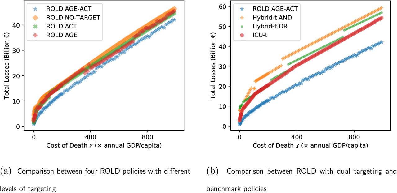
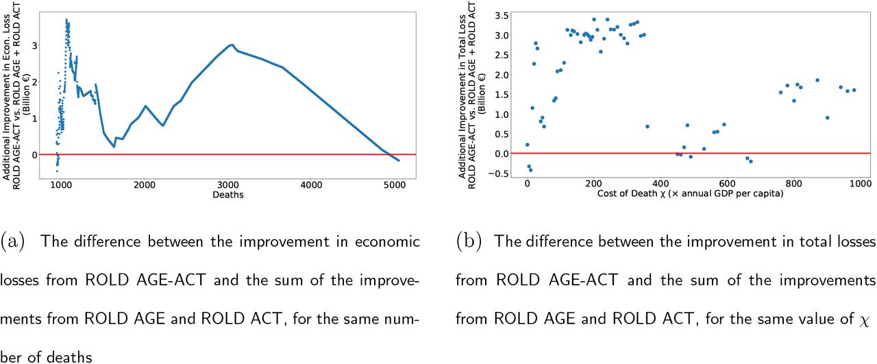
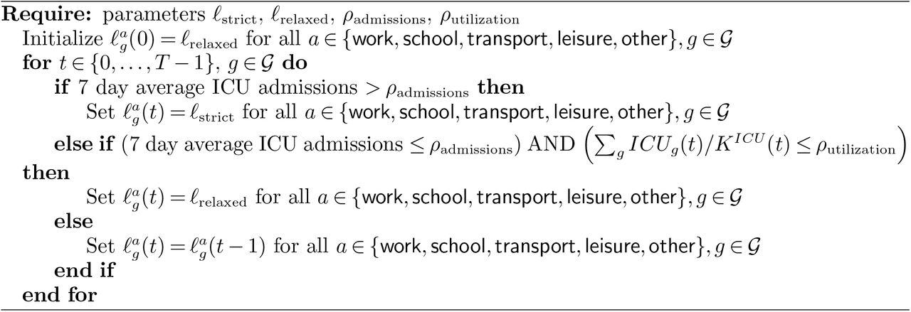
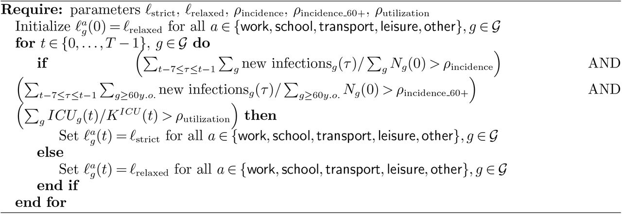
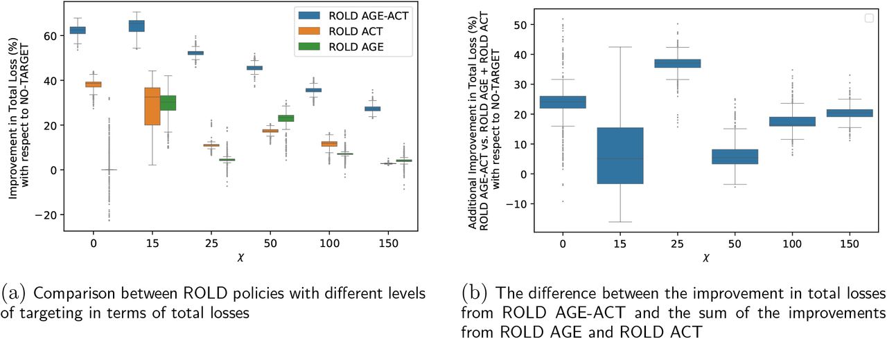