
Abstract
Accurate computational models for clinical decision support systems require clean and reliable data, but in clinical practice, data are often incomplete. Hence, missing data could arise not only from training datasets but also test datasets which could consist of a single undiagnosed case, an individual. Many popular methods of handling missing data are unsuitable for handling such missing test data. This work addresses the problem by evaluating multiple imputation and classification workflows based not only on diagnostic classification accuracy but also computational cost. In particular, we focus on dementia diagnosis due to long time delays, high variability, high attrition rates and lack of practical data imputation strategies in its diagnostic pathway. We identified and replicated the extreme missingness structure of data from a memory clinic on a larger open dataset, with the original complete data acting as ground truth. Overall, we found that computational cost, but not accuracy, varies widely for various imputation and classification approaches. Particularly, we found that iterative imputation on the training dataset combined with a reduced-feature classification model provides the best approach, compromising speed and accuracy. Taken together, this work has elucidated important factors to be considered when developing or maintaining a dementia diagnostic support system, which can be generalized to other clinical or medical domains, particularly with extreme data missingness.
I. Introduction
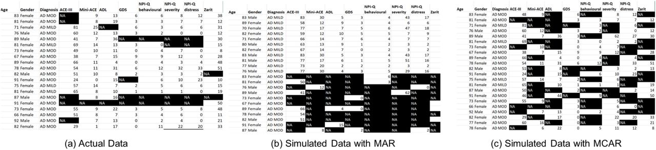
Computerized decision support tools for clinical decision making can enhance consistency, objectivity and standardization [2]. In developing a diagnostic model, a large complete training dataset is typically used to build a classification model, while a test dataset is used to verify model accuracy [3]. However, actual clinical data can appear very different from well-curated data. In particular, data in clinical practice contains a lot of missing values (see Fig. 1a) [4]–[6]. In fact, the issue of missing data is one of the most ubiquitous concerns in data science [7]. Hence, computational models used in clinical decision support systems must incorporate a strategy for handling missing data.

Sample Alzheimer’s disease (AD) dataset from a memory clinic and its breakdown of data missingness. (a) Initial sample data. Rows: patients; columns: diagnosis category (AD MILD or AD MOD for mild or moderate AD, respectively), the various cognitive and functional assessments, Gender and Age. Black cells with “NA” label: missing data. (b-c) Simulated data with missingness correlated with diagnosis (Missing at Random, MAR) (b), and uncorrelated with any variable (Missing Completely at Random, MCAR) (c).
Current strategies for handling missing data include: (i) complete-case analysis, in which any row with a missing value is dropped from analysis; (ii) data imputation, in which missing values are replaced with an estimated value; (iii) missing-indicator methods, in which missing values are marked as missing and then incorporated in the training dataset; and (iv) various strategies in which missing data is tackled directly in the analysis without an intermediate imputation step [8]–[10]. The latter include maximum-likelihood methods [11], classifiers which can account for the uncertainty caused by missing data such as the naïve credal classifier [12], and tree-based classifiers which use the surrogate split method [13]. Data imputation strategies can further be divided into single imputation methods, in which a single estimate for the missing data is generated, and multiple imputation methods, which generate multiple estimates for each missing value and therefore will produce multiple imputed datasets for further analysis [4], [14].
The appropriate strategy for dealing with missing data will depend to some extent on the type of missingness. Missing data is often categorized into three types: missing at random (MAR); missing completely at random (MCAR); and missing not at random (MNAR) [15]. In the case of MAR, the probability that data is missing depends upon the variables observed within the dataset – e.g. if the variable of gender has been observed in a survey, and women are more likely to complete the survey (Fig. 1b). MCAR can be understood as a special case of MAR – in this case, the probability of missingness is independent of all variables in the dataset. An example would be someone being late for a medical appointment because of a traffic jam and their data is not recorded (Fig. 1c). MNAR is the case where the probability of missingness depends on a variable which is in itself missing; this is the most complex case to handle. An example of this might be a survey on income, in which people with a very low or very high income refuse to report their income [4].
In practice, clinical data tends to have MAR type missingness [4]. However the probability of missingness in clinical data is often dependent on the outcome variable, as illness/disease severity may impact opportunities for data gathering [16]. In longitudinal data, this may be MNAR type missingness, such as the case where a study participant may not be able to undergo a specific assessment or be part of a follow up study due to an increase in disease severity. The correlation between missingness and disease severity holds true in dementia data, as shown in [17].
Various studies have evaluated different imputation methods for replacing missing values in clinical data [4], [14], [18]–[21]. The most effective methods are found to be multivariate, iterative methods such as Multiple Imputation by Chained Equations (MICE) [20] fuzzy k-means [14], [18], Bayesian Principal Component Analysis [18] and missForest [22], and more recently, unsupervised neural network’s autoencoders [23]. However, most studies are focused on handling missingness in the training dataset, despite the fact that the test dataset can have missing values. For example, the diagnosis of a patient may involve unknown data variables from that patient (Fig. 2).
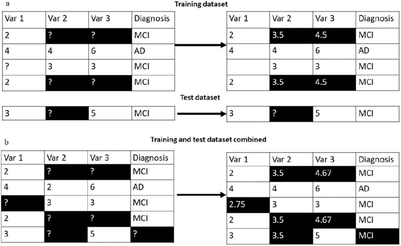
Iterative imputation with single-row test dataset. Iterative imputation begins with mean imputation. (a) A toy example where training dataset and test dataset are imputed separately. It is impossible to impute the missing values in the test dataset, because we have no way to compute the mean of the variables which are missing. (b) Same example in (a) but using combined imputation of training and test datasets
The case of missing values in the test dataset during classification was addressed in [24], which also notes the dearth of literature on this issue. Specifically, [24] delineated four different strategies for handling the situation of missing values in the test data: (i) discarding objects with missing values; (ii) acquiring the missing value through manual follow-up; (iii) data imputation; or (iv) using a reduced-feature classification model built with variables which are not missing in the test dataset. The study concluded that reduced-feature models are the most effective solution to this problem. Another study evaluated strategies for missing values in the test dataset in the context of a tree-based classifier and for eight different missing data patterns, using simple datasets with a binary response variable [25]. The conclusion was that a missing-indicator method was the most useful where missingness is related to the response variable. A later study [26] directly addressed the problem of missing values in the test clinical dataset, using k-nearest neighbors (k-NN) imputation method [27] to impute the dataset before testing the impact on classification accuracy.
It is clear that the above studies for handling missing test data are limited. Specifically, [24] and [25] had yet to test their methods on actual clinical data, and did not discuss the issue of missing training data, while the workflow in [26] may potentially fall into the pitfall known as “double-dipping” [28] as training and test datasets were imputed together. In particular, for clinical decision making, many of these current methods of handling missing data are unsuitable for handling a test dataset which consists of a single case (e.g. representing a single patient) (Fig. 2). There is no recommendation in the literature on how to handle missing values in the condition where an individual test case, which may have missing data, is evaluated. Additionally, very little missing data literature deals with extreme (i.e. high proportion of) missingness. Crucially, almost no literature deals with significant missingness in both training and test datasets, although in real life both training and test datasets are frequently drawn from the same population with similar proportion of missing data.
In this paper, we address the above issues by proposing a novel workflow for a clinical decision support system that takes into account the realities of clinical data and the leave-one-out cross validation (LOOCV) condition more suitable for clinical decision-making. We focus on the diagnosis of dementia, particularly Alzheimer’s disease (AD), due to AD being the most common form of dementia, and AD’s long time delays and high variability in its diagnostic pathway [1]. Importantly, longitudinal studies on cognitive decline have high attrition rates (e.g. [29]–[31] and there is a substantial lack of practical data imputation strategies for dementia diagnosis (e.g. [1], [32]–[39]). In this work, we propose practical strategies that handle widespread missing test data with missing patterns that resemble that from actual memory clinical data. Through investigating various strategies we shall demonstrate that imputation accuracy does not necessarily correlate with classification accuracy and that Random Forest (RF) imputation on the training dataset, combined with a reduced-feature classification model, provides the most effective solution.
II. Methods
A. Data Description
1) Clinical Dataset to Extract Missing Data Characteristics
Anonymous clinical data were extracted from Altnagelvin Area Hospital’s Memory Assessment Service (WHSCT). Ethics approval for this was obtained from the Office for Research Ethics Committee Northern Ireland (ORECNI, HSC REC B reference: 17/NI/0142; IRAS project ID: 230077). This data was used to extract the type of missingness in actual clinical dataset. Based on text-based diagnosis from clinicians, AD diagnosis was manually categorized into two classes, AD MILD (mild AD) and AD MOD (moderate AD). Other diagnostic categories were discarded due to lack of ordinality or their small sizes. A sample of the resulting dataset is shown in Fig. 1A. There are 189 rows in total, with each row representing a patient. Cells with missing values are shown in black in the diagram. Features in the clinical data consist mainly of cognitive and functional assessments (CFAs).
In our previous work, we have shown that CFAs are among the most predictive features for classifying AD severity [40], [41]. For the current clinical dataset, the CFAs included Addenbrooke’s Cognitive Examination (ACE-III) and the Mini-ACE [42], the Bristol Activities of Daily Living Scale [43], the Geriatric Depression Scale [44], the NPI-Q behavioral, distress and severity measurements [45], and the Zarit Caregiver Burden [46]. Hence, this study will focus on CFA features. The extracted missingness structure of this dataset will be replicated in a complete open source dataset, as described below.
2) ADNI Dataset
The data for evaluating the missing data strategies was extracted from the ADNIMERGE table [47] from the Alzheimer’s Disease Neuroimaging Initiative (ADNI) merge R package, which amalgamates several key tables from the ADNI open source dementia data (adni.loni.usc.edu). The ADNI open database included clinical and neuropsychological assessments with diagnosis labelled as healthy, mild cognitive impairment (MCI) and early AD. It should be noted that the MCI group may include prodromal stage of AD, and individuals who will not progress to AD.
The CFAs in the ADNIMERGE dataset after feature selection (see section II.B.1) was applied were: Mini-Mental State Examination (MMSE) [48]; Alzheimer’s Disease Assessment Scale 13 (ADAS13) [49]; Montreal Cognitive Assessment (MoCA) [50]; Logical Memory – Immediate Recall (LIMMTOTAL) [51]; Logical Memory – Delayed Recall (LDL TOTAL) [51]; Rey Auditory Verbal Learning Test (RAVLT): Immediate, Learning, Forgetting, and Perc Forgetting, [52]; and Functional Assessment Questionnaire (FAQ) [53]. We also included Gender and Age in our analysis, mirroring the clinical dataset.
We make use of CDR-SB (Clinical Dementia Rating Sum of Boxes) instead of the more subjective clinical diagnosis [54]. CDR-SB was re-coded from the ADNI variable CDR (Clinical Dementia Rating) following the protocol in [55]. The mild, moderate and severe AD classes were amalgamated creating a three-class outcome variable: Healthy Controls (HC), MCI, and AD.
Importantly, we used the resulting ADNIMERGE data to: (i) create synthetic missing datasets from a complete ADNI dataset, based on the missingness structure of actual clinical data as described in Section II.A.1; (ii) evaluate the various computational approaches; and (iii) develop our proposed workflow.
B. Computational Methods
1) Feature Selection
Feature selection was performed on the ADNIMERGE table using the information gain (IG) algorithm [56], which is described by
 where H is Shannon’s entropy [57] defined by
 in which P is the probability function of some random variable X for possible outcomes Xi. H is equal to the sum of the probability of each label multiplied by the log probability of each label and can be understood as a measure of “disorder”, with a value ranging between 0 and 1. IG of a given attribute is the reduction in disorder of the class variable, when the class variable is separated according to that attribute.
The 8 CFAs which had the highest IG with respect to the CDR-SB outcome variable were selected. In addition, the MMSE score was retained to facilitate mapping of the types of missingness from the clinical dataset, as described in Section II.B.2. Rows with missing values for any of these features were dropped, creating an initial complete ADNIMERGE dataset with 1185 rows (the base dataset), with each row representing one individual. This base dataset provides the ground truth for our study. Synthetic missing datasets were derived from this dataset for imputation and classification testing.
2) Missing Data
Next, we searched for the relationship between missing values and the degree of cognitive decline of the individual/patient. Although no CFA in ADNIMERGE can be found in the clinical dataset, a previous study has provided a table of conversion between ACE-III scores (in our clinical dataset) and MMSE scores (in ADNIMERGE) [58]. In particular, these two CFAs were temporarily used to map the missingness structure from the clinical dataset to ADNIMERGE but subsequently not considered in the analysis (see below). We used the ACE-III scores in our clinical dataset as the benchmark for the relationship between missingness and cognitive decline, to facilitate this mapping without using the outcome variable for generating missingness (which would create double-dipping in subsequent analysis).
We first performed a regression of the probability of missingness in the clinical dataset on ACE-III. The resultant regression equation (see Section III.1) was then used to generate synthetic missing data in the ADNIMERGE dataset. Specifically, the MMSE score in ADNIMERGE was converted into an ACE-III score using the conversion table in [58]. Missing values were then synthetically introduced into the CFA variables in the ADNIMERGE dataset using this conversion. We showed, in Section III.A, that the proportion of missing data for CFA values was very high. Thus, in total, 10 synthetic ADNIMERGE datasets with different random missing patterns were generated, to ensure robustness in the results. ACE-III and MMSE scores were dropped from subsequent analysis, because ACE-III was not in ADNIMERGE and MMSE was not selected by feature selection.
3) Data Imputation Methods
We included traditional mean and median data imputation methods [7] for analysis as they are straightforward to interpret and can function as a benchmark. We also used a multiple imputation method termed Predictive Mean Matching (PMM) [59]–[62] from the multivariate imputation via chained equations (MICE) package in R [63]. We used PMM both in the form of a single imputation (PMM1) and the mean of 5, 10, 15 and 50 imputations (PMM5, PMM10, PMM15 and PMM50, respectively). It should be noted that PMM is the default method for MICE, the most commonly used multiple imputation package. Imputation algorithms such as the k-NN method [27] which generalize from complete cases, were unsuitable for our high proportion of missing data, and were not considered.
The general steps for PMM are as follows [62]: (i) perform a linear regression for 2 variables with no missing data, and obtaining a set of coefficients; (ii) make a random draw from the posterior predictive distribution of this set of coefficients, creating a new set; (iii) using the newly generated coefficients to generate predictive values for all cases, on data with and without missingness; (iv) identify a set of cases with observed variable whose predicted values are close to the predicted value for the case with missing data; and (v) from these cases, randomly choose one case and assign its observed value to substitute for the missing value. Steps (ii) to (v) are then repeated until the dataset is filled with values, i.e. complete. For PMM1, there is only 1 case in step (iv), while there are 5 cases for PMM5.
Another algorithm which we used was the iterative missForest [22] from the missForest package in R [64], which uses Random Forest (RF) regression to impute missing data [65]. The missForest imputation method was chosen as it had been shown to outperform MICE at imputation [22], [66] and involved few assumptions about the structure of the missing data [22]. The MissForest method entails the following steps: (i) impute the column mean for each missing value in dataset D to create imputed dataset D’; (ii) copy D’ to D’’; (iii) for each column in D’ use the rows with no missing values to build a RF model, and use the model to predict the missing values; (iv) update D’ with new predictions for the missing values; (v) test convergence and output D’’ if convergence is reached – if maximum iterations have been reached output D’; otherwise iterate steps (ii-v).
Finally, we also used the Bayesian Principal Components Analysis (BPCA) [67] algorithm for imputation as it has been found to be effective in previous studies [18], and in order to explore whether a PCA based method impacts imputation accuracy by variable. Bayesian PCA is a computationally complex method which uses an iterative approach similar to Expectation Maximization, combined with Bayesian modelling to estimate the eigenvalues of the underlying principal components of the dataset.
The adjusted R2 of the linear regression of the imputed values on ground truth (complete data) was used as a measure of imputation accuracy, with values ranging from 0 to 1 (poorest to highest in accuracy, respectively). The mean, minimum and maximum R2 measurements from each of the 10 synthetic datasets were obtained. This methodology was also used to calculate the average imputation accuracy of each variable using the missForest algorithm.
The computation time over 10 missing datasets for each imputation method was recorded and normalized by dividing by the time for the fastest method (mean imputation)
4) LOOCV Classification Accuracy Testing
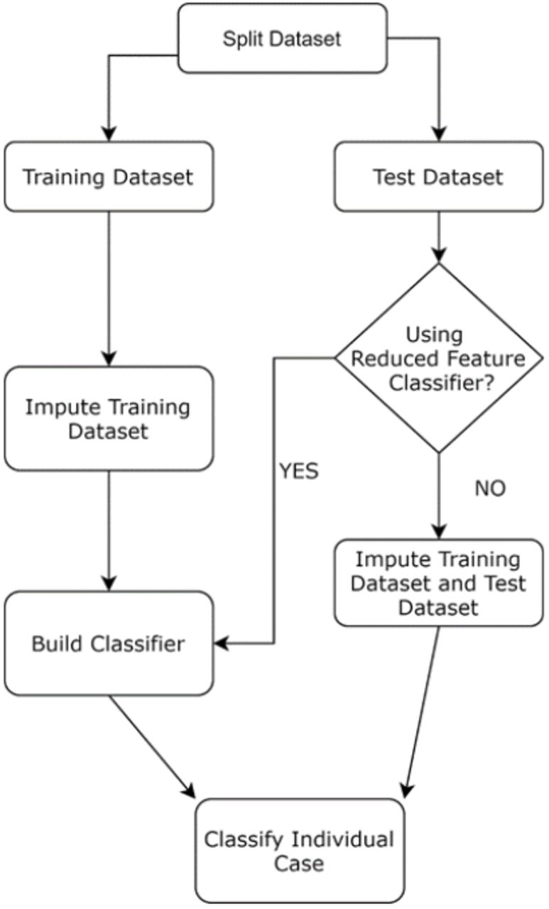
Classification accuracy was tested using leave-one-out cross-validation (LOOCV) [69]. In the LOOCV condition, the test dataset is only one row. We used LOOCV to mimic one-patient classification condition. Further, LOOCV is suitable for smaller data sizes, which may occur in some clinical/medical centres. Although LOOCV is computationally intensive, it minimizes model bias by using almost all the training data for each classification while allowing conservative estimation [70]. The approaches we used for handling missing values in the test row can broadly be divided into two categories: 1) impute the missing values in the test row using the imputation approach used for the training dataset; or 2) use a reduced-feature classifier, where a classification model is built using only the features which are not missing in the test row. In a dataset with N rows, a classification model will be built N times and tested on each row in turn. A schematic of this process is shown in Fig. 3.

Workflow for LOOCV (single case) classification testing, emulating actual clinical decision-making conditions. Data is first split into training and single-case test datasets. The training dataset is imputed separately from the test dataset.
The following 16 workflows were tested: (A) mean imputation of training and test datasets, RF classifier; (B) imputation of the training dataset by class mean with reduced-feature RF classifier; (C) imputation of training and test dataset by missForest with RF classifier; (D) mean imputation with reduced-feature RF classifier; (E) RF imputation of training and test dataset with reduced-feature RF classifier; (F) PMM-5 multiple imputation of training and test dataset, with the modal value imputed to the outcome variable in the test dataset used as the estimated class; (G) PMM-5 imputation of training and test datasets with the modal output of 5 RF classifiers built with the 5 imputed training datasets used as the estimated class; (H) naïve Bayes classifier [71] from the e1071 R package [72], with no attempt to impute training or test dataset; (I) PMM-5 imputation of training dataset with the modal output of 5 reduced-feature RF classifiers used as the estimated class; (J) mean imputation of training and test dataset with linear support vector machine (SVM) classifier [73] from the e1071 R package; (K) RF imputation of training and test datasets with linear SVM classifier; (L) RF imputation of training dataset with reduced feature linear SVM classifier; (M) imputing both training and test dataset with the mean of PMM-15, RF classifier; (N) imputing training dataset with the mean of PMM-15, reduced-feature RF classifier; (O) imputing both training and test dataset with the mean of PMM-15, SVM classifier; and (P) imputing training dataset with the mean of PMM-15, reduced feature SVM classifier.
The RF classifier was used in most cases, as it is versatile and adaptable to a wide variety of different datasets [22], with the SVM classifier used in some workflows to test whether imputation strategies have different compatibility with different classifiers. The naïve Bayes classifier was used in (H) as it does not require a strategy for handling missing values; the classifier can skip a missing value while still making use of values in the same row of the dataset due to the conditional independence assumptions in the naïve Bayes algorithm. The RF imputation method was used as it was the most effective single imputation method, as well as multiple imputation with PMM-5 (higher values of multiple imputation were not considered here due to the impact on classification speed) and single imputation with the mean of PMM-15, which although not intended for single imputation was found to be both faster and more accurate as an imputation method than RF.
The percentage of correct classifications in each workflow over the 1185 cases was recorded. In a clinical decision support setting, imputation and classification will occur in different contexts, so the computation times for imputation and classification in each workflow were recorded separately. The mean computation time for each of the 1185 classification and imputation cases was recorded.
C. Software and Hardware for Analysis
The above analyses and algorithms were run within R Studio version 1.146 on a Windows machine with R version 3.5.2 installed.
III. RESULTS
A. Synthetic missing data with missingness type from clinical data
To reduce the size of the ADNIMERGE dataset to better resemble the clinical dataset, we performed feature selection we performed feature selection using the information gain algorithm [56] which selects the best features with respect to the class variable (CDR-SB scores in our case), and identified the 8 most relevant CFA features. Table I shows the selected CFAs in descending order of their information gain against the class variable. Interestingly, most of the selected CFAs were completed by study partners, as opposed to being completed by patients themselves (Table I, column 2). Next, we use the top 8 CFAs, plus Gender and Age variables and our class variable from the ADNIMERGE data to form our baseline dataset which resembles the types of features in the memory cslinic data. We then investigate the missingness in our memory clinic data, in order to reproduce the same missingness patterns in the ADNIMERGE data.
Features Selected by Information Gain
We first perform a regression of the probability of any given value being missing in the memory clinic data, on the degree of cognitive decline as measured by Addenbrooke’s Cognitive Examination (ACE-III). We do not use the outcome variable as the measurement of cognitive decline for this regression. This is because the regression will be used to generate missingness in the ADNIMERGE dataset and basing it on the outcome variable would create the potential for double-dipping. ACE-III scores can be mapped onto MMSE scores [58] thus creating a link between ADNIMERGE and our clinical dataset. Hence ACE-III is chosen as our measure of cognitive decline in the clinical dataset.
We found that the resulting regression equation can be described by Pmiss = 0.48 + (0.06 ACE-III), where Pmiss is the probability of any given value being missing, and ACE-III consists of its normalized score. The 0.48 constant in the equation means that 48% of the CFA values are missing. The low p-value (2×10⁻¹⁶) and low R2 (0.02502) of the regression indicate that cognitive decline is a weak predictor of missingness, suggesting a MAR type missingness. Using this regression, and a conversion table to convert ACE-III scores in the clinical dataset to MMSE scores in ADNI [58] we created 10 synthetic missing datasets from the original complete ADNIMERGE data with the same degree and type of missingness as in our clinical data (see Section II.A.2).
B. Computationally expensive imputation methods are not necessarily more accurate
Based on the synthetic missing datasets, we performed various imputation methods. We found that the Predictive Mean Matching (PMM) and Random Forest (RF) imputation methods provided the highest accuracy when tested against the complete dataset (ground truth) (Fig. 4). PMM imputation methods were further divided into PMM5, PMM10, PMM15, PMM50 - the mean of 5, 10, 15 and 50 multiple imputations, respectively. Specifically, the regression of the mean of the PMM50 imputation method against ground truth was the most accurate, with a mean R2 over 10 synthetic datasets of 0.86 (Fig. 4). This was non-significantly (p=0.204) higher than the accuracy when using PMM15 imputation (mean 0.861), but significantly higher than the accuracy for PMM10 (0.856) (t-test p-value over 10 datasets = 0.002). The PMM15 method was in turn significantly (p=0.001) more accurate than the RF method (mean 0.849) although the RF was the only method with accuracy close to the PMMs. Thus, PMM’s accuracy marginally increased when more multiple imputations were generated. All PMM methods involving more than 15 imputations were significantly more accurate than RF.
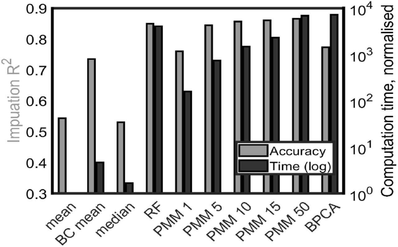
Imputation accuracy R2 and computation time depend on imputation methods. Grey (black) bars: accuracy R2 (computation time). Left-to-right bars: mean imputation, mean by class imputation, median imputation, RF imputation, PMM averaged over 1, 5, 10, 15 and 50 imputations, and BPCA.
The next most accurate method, Bayesian Principal Component Analysis (BPCA), was found to have an accuracy R2 of 0.773. The BC mean (mean by class) imputation method had a reasonable accuracy for a computationally simple method (R2=0.735), but as an imputation method it has the disadvantage that it cannot be used to impute the test row as the class value of the test row is not known. Finally, the median and mean methods did not achieve high accuracy.
Given that many of the mean R2 values were between 0.8-0.9 (Fig. 4, grey bars), we next investigated the computational cost of individual imputation methods. We found that there was a wider range of computational times across the various imputation methods (Fig. 4, black bars; note the logarithmic scale). In particular, BPCA and PMM50 had similar timescales, while RF was about twice as fast. PMM15 was twice as fast as RF. The mean, BC mean and median methods, as might be expected, were not computationally costly. Overall, computationally expensive methods can achieve higher accuracy than simpler methods (e.g RF and PMMs cf. mean, median and BC median), but algorithmic complexity does not guarantee high accuracy (e.g. BPCA)
C. Running time varies logarithmically across approaches
Next, we investigate the most effective data imputation methods in a clinical decision support setting, with respect to classification accuracy and computational cost. We test various workflows A-P (Table II) for classification and imputation of training and test datasets in the LOOCV condition, where each case in the dataset is classified one at a time, mimicking handling a single patient/individual (Section II.B.4). To demonstrate this, it suffices to use just one of the synthetic datasets. The test dataset, consisting of only 1 row, is imputed either with the same imputation algorithm as the training dataset, or is not imputed and is classified using a reduced-feature classifier which uses only features which are not missing in the test dataset.
Imputation and Classification Workflows
Among the workflows we tested, we find that the highest 3-class classification accuracy is limited to 79%. This is a surprising result, given the extreme (48%) missingness that was introduced. Workflows which fell short of this accuracy include F, H and K and, to a lesser extent, N and P. We suggest that perhaps these workflows should be ruled out for practical use. Specifically, F, with 74% accuracy, does not use a conventional classifier, while workflow H, using naïve Bayes algorithm, attains only 71% accuracy. This is unsurprising as naïve Bayes algorithm relies on the assumption that features in the dataset are conditionally independent given the outcome variable. For workflow K, a mean imputation combined with SVM classifier, the low accuracy is unsurprising given the low accuracy of mean imputation. Workflows N and P use the PMM15 mean imputation method in combination with the reduced-feature method for test data, and by contrast with the combination of RF imputation and the reduced-feature method, this combination does not reach the maximum accuracy for this dataset. Overall, we found that the average sensitivity and specificity for all the workflows for combined MCI and AD classes are both around 76%, with workflow H having the lowest specificity (59%).
Given that no approach stands out in terms of accuracy, we then investigate the computation time. In particular, the running time for the LOOCV workflows has been divided into classification time (time to build the classifier and perform classification) and imputation time (time to impute the training set) presuming that in a clinical decision support system, imputation is performed during off-peak times. Hence, workflows C, F, G and K, with test dataset imputed iteratively alongside the training dataset, may be impractical for use in clinical decision-making setting (Fig. 5) and can also be ruled out for practical use – these are included only for benchmarking purposes.
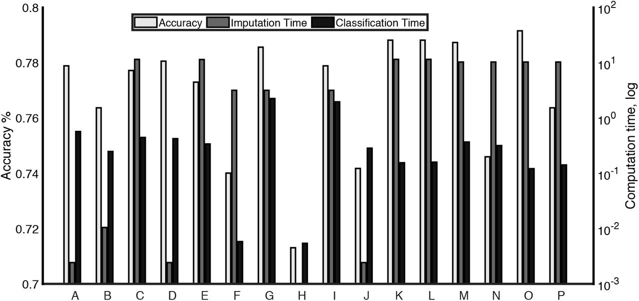
Imputation and classification workflows evaluated for classification accuracy (grey, left axis; linear scale), imputation time and classification time (black, right axis; logarithmic scale.) The details of the workflows are explained in Table 2.
Methods which maximise accuracy and are computationally practical are A,B,D,E,I, L, M and O, although it should be noted that Method I, which uses a multiply imputed dataset and a RF ensemble classifier, is significantly more expensive in classification time without offering any accuracy improvement over A,B,D,E and L. The accuracy of workflow A (mean imputation and RF classifier) is notable in contrast with workflow K, which uses mean imputation in combination with an SVM classifier.
IV. DISCUSSION
Clinical datasets such as in electronic health records often have a significant proportion of missing data [5], [6]. Various strategies have previously been proposed, however there is no study in the literature that deals with the practical problem of missing dementia data in the test dataset, even though this is a very likely problem to occur in clinical practice. This “test dataset” is the individual patient who is being diagnosed and it is highly likely that there could be incomplete information about any given patient. Missing data in the test dataset may prohibit the use of many popular imputation methods, which are frequently iterative and computationally costly when datasets are large. In this work, with a focus on AD diagnosis, we have replicated the missingness structure of a real (memory) clinical dataset and proposed practical strategies for dealing with large amount (48%) of missing data in training and test datasets (Fig. 2). Moreover, we evaluated the approaches under LOOCV condition (Fig. 1), mimicking real-world clinical decision-making (Fig. 3). Overall, we found that various strategies for imputation and classification in these conditions were able to maximise the classification accuracy but these methods vary widely in computation time (Figs. 5 and 6) and this is likely to be an important factor to be considered when developing or maintaining a clinical decision support system.
In particular, reduced-feature methods for dealing with missing test datasets were equally accurate to methods that involved imputing the test dataset, but this is sensitive to the imputation method. Reduced-feature methods may be the best solution for building a clinical decision support tool with large data as they do not involve real-time imputation of the test dataset. Specifically, we found RF imputation of the training dataset combined with a reduced-feature SVM classification (workflow L in Table II) reached optimal accuracy and was also the fastest classifier to build.
Mean imputation combined with an RF classifier performed surprisingly well in our testing despite the low accuracy of mean imputation (Fig. 4.) Indeed, mean imputation of training and test set combined with a reduced feature outperformed all the other workflows for balanced accuracy (75.4%). When real-time computational speed is at a premium and the dataset has large number of features, it may be worth considering using mean imputation of the training and test datasets combined with RF classification (workflow A). This holds true despite the low accuracy of mean imputation (Fig. 4). Notably, mean imputation combined with an SVM classifier led to low classification accuracy. It may be the case that accurate imputation is not necessary for accurate classification when a decision tree classifier e.g. RF is used [25].
Supporting the finding that increasing imputation accuracy does not necessarily increase classification accuracy are the results using imputation by PMM15. Multiple imputations are typically classified using a pooled classifier that classifies each instance of the dataset separately, but this is computationally costly in classification time (Fig. 6/Table II, workflows I and G). Taking a mean over the results of multiple imputation is not a conventional imputation method, but our study found this method to be computationally faster (for PMM15, PMM10 and PMM5 conditions) and more accurate (for PMM15 and PMM50 conditions) than the most effective single imputation method (RF). However, when datasets imputed this way were used for classification the accuracy seemed lower than the accuracy of RF imputed datasets when reduced-feature classification was used.
Our present study has several limitations and could be extended in several ways. So far, we have only used one dataset from a memory clinic. In future studies, different clinical datasets with different types of clinical features will need to be explored to validate our results. Moreover, we have only investigated an extreme case of missingness of the MAR type. Future work will investigate whether this novel approach could be extended to cases with less, and different types of missingness. We have also not completely evaluated other imputation methods, such as those using unsupervised learning with autoencoders [23]. Their performance should be compared with the methods used in our current study. In conclusion, we have developed a computational framework for handling missing test data for practical clinical applications. Our framework is sufficiently general to be applied to other data types.
Data Availability
Data from the Alzheimer's Disease Neuroimaging Initiative (ADNI) is openly available.
ACKNOWLEDGEMENTS
Data collection and sharing for this project was funded by the Alzheimer’s Disease Neuroimaging Initiative (ADNI) (National Institutes of Health Grant U01 AG024904) and DOD ADNI (Department of Defense award number W81XWH-12-2-0012). ADNI is funded by the National Institute on Aging, the National Institute of Biomedical Imaging and Bioengineering, and through generous contributions from the following: AbbVie, Alzheimer’s Association; Alzheimer’s Drug Discovery Foundation; Araclon Biotech; BioClinica, Inc.; Biogen; Bristol-Myers Squibb Company; CereSpir, Inc.; Cogstate; Eisai Inc.; Elan Pharmaceuticals, Inc.; Eli Lilly and Company; EuroImmun; F. Hoffmann-La Roche Ltd and its affiliated company Genentech, Inc.; Fujirebio; GE Healthcare; IXICO Ltd.; Janssen Alzheimer Immunotherapy Research & Development, LLC.; Johnson & Johnson Pharmaceutical Research & Development LLC.; Lumosity; Lundbeck; Merck & Co., Inc.; Meso Scale Diagnostics, LLC.; NeuroRx Research; Neurotrack Technologies; Novartis Pharmaceuticals Corporation; Pfizer Inc.; Piramal Imaging; Servier; Takeda Pharmaceutical Company; and Transition Therapeutics. The Canadian Institutes of Health Research is providing funds to support ADNI clinical sites in Canada. Private sector contributions are facilitated by the Foundation for the National Institutes of Health (www.fnih.org). The grantee organization is the Northern California Institute for Research and Education, and the study is coordinated by the Alzheimer’s Therapeutic Research Institute at the University of Southern California. ADNI data are disseminated by the Laboratory for Neuro Imaging at the University of Southern California.
Footnotes
This work was supported by the European Union’s INTERREG VA Programme, managed by the Special EU Programmes Body (SEUPB), and additional support by Alzheimer’s Research UK (XD, MB, ST, PLM., KW-L), Ulster University Research Challenge Fund (XD, MB, ST, PLM, KW-L), and the Dr George Moore Endowment for Data Science at Ulster University (MB). The views and opinions expressed in this paper do not necessarily reflect those of the European Commission or the Special EU Programmes Body (SEUPB).
(k.wong-lin{at}ulster.ac.uk)
References
- [1].↵
- [2].↵
- [3].↵
- [4].↵
- [5].↵
- [6].↵
- [7].↵
- [8].↵
- [9].
- [10].↵
- [11].↵
- [12].↵
- [13].↵
- [14].↵
- [15].↵
- [16].↵
- [17].↵
- [18].↵
- [19].
- [20].↵
- [21].↵
- [22].↵
- [23].↵
- [24].↵
- [25].↵
- [26].↵
- [27].↵
- [28].↵
- [29].↵
- [30].
- [31].↵
- [32].↵
- [33].
- [34].
- [35].
- [36].
- [37].
- [38].
- [39].↵
- [40].↵
- [41].↵
- [42].↵
- [43].↵
- [44].↵
- [45].↵
- [46].↵
- [47].↵
- [48].↵
- [49].↵
- [50].↵
- [51].↵
- [52].↵
- [53].↵
- [54].↵
- [55].↵
- [56].↵
- [57].↵
- [58].↵
- [59].↵
- [60].
- [61].
- [62].↵
- [63].↵
- [64].↵
- [65].↵
- [66].↵
- [67].↵
- [68].
- [69].↵
- [70].↵
- [71].↵
- [72].↵
- [73].↵
- [74].


