
Abstract
Real-time estimates of the true size and trajectory of local COVID-19 epidemics are key metrics to guide policy responses. We developed a Bayesian nowcasting approach that explicitly accounts for reporting delays and secular changes in case ascertainment to generate real-time estimates of COVID-19 epidemiology on the basis of reported cases and deaths. Using this approach, we estimate time trends in infections, symptomatic cases, and deaths for all 50 US states and the District of Columbia from early-March through June 11, 2020. At the beginning of June, our best estimates of the effective reproduction number (Rt) are close to 1 in most states, indicating a stabilization of incidence, but there is considerable variability in the level of incidence and the estimated proportion of the population that has already been infected.
One Sentence Summary A new method to track epidemiologic measures of COVID-19, available in the covidestim package for R.
Main Text
The number of newly-diagnosed cases and confirmed COVID-19 deaths are the most easily observed measures of the health burden associated with COVID-19. However, the early response to COVID-19 in the United States (US) was hindered by limited access to reliable diagnostics (1). Because of these limitations, the number of reported cases and deaths over this period will have underestimated the true size of the epidemic, with some individuals developing, and potentially dying from, COVID-19 without receiving a lab-confirmed diagnosis (2). Furthermore, while the number of cases and deaths describes the magnitude of health effects, they are a lagged indicator of the transmission dynamics of the pathogen, affected by delays associated with the disease incubation period, care-seeking behavior of symptomatic individuals, diagnostic processing times, and reporting practices.
Near real-time estimates of the size and trajectory of the local COVID-19 epidemic are key metrics to guide state-level policy about stay-at-home orders and physical distancing recommendations. Ideally, information describing trends in transmission, rather than trends in reported cases or deaths, would be available to track the impact of disease control efforts. A key metric for describing transmission changes is the effective reproduction number (Rt), which represents the average number of secondary cases caused by a case at a given point in time. An Rt less than 1 indicates a declining epidemic, while an Rt greater than 1 indicates a growing epidemic (3). The delayed and incomplete nature of reported cases and deaths means that these observable outcomes are not ideal for producing reliable estimates of Rt. Moreover, rapid changes in testing practices can bias Rt estimates generated from raw surveillance data, making it difficult to understand the current trajectory of local outbreaks and the effects of interventions (4).
Here, we present a method to estimate the daily incidence of new SARS-CoV-2 infections from observed case notification and death reports. We apply our model to publicly available COVID-19 case, death, and testing data for all 50 U.S. states and the District of Columbia. The model is available on GitHub and through the covidestim package for the R programming language.
We estimate COVID-19 epidemiological outcomes from reported time-series of cases and deaths, using a mechanistic model to account for changes in case ascertainment that result from fluctuating availability of diagnostics, as well as delays associated with disease progression, diagnosis, and reporting systems. We estimate infections, cases (symptomatic infections), deaths, and detected and reported cases (Fig. 1) and deaths (Fig. S1). Ascertainment of COVID-19 cases was estimated to vary considerably across states. We estimate that the percentage of detected cases (estimated cumulative cases divided by cumulative detected cases) ranged from 13.2% (95% uncertainty interval: 6.0%, 28.2%) in Arizona to 41.7% (22.4%, 62.5%) in Wyoming as of June 11, 2020. The estimated fraction of COVID-19 deaths detected ranged from 77.4% (59.4%, 85.7%) in Wyoming to 82.0% (42.3%, 90.0%) in New York as of June 11, 2020.
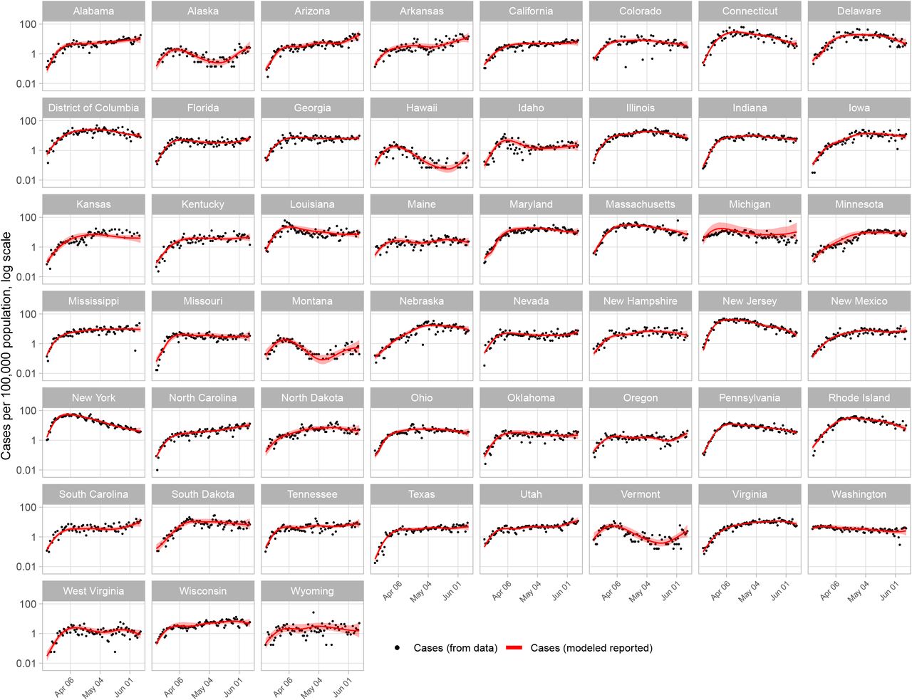
Model estimates and empirical data for reported COVID-19 cases by state, log scale. Values are per 100,000 population, from March 15 to June 11, 2020. Empirical values not shown for days with zero reported cases.
The state with the greatest number of estimated new infections in a single day was New York, with 112,838 (58,816, 281,042) on March 17, equivalent to 580 (302, 1,445) new infections per 100,000 population (Fig. 2). The majority of states saw a peak in new infections sometime between mid-March and early-April and have experienced flat or declining incidence between mid-April and early-June. Notable exceptions to this trend include Arizona, where we estimate new infections have been increasing steadily since early April, and Georgia, where we estimate new infections plateaued at the end of March (Fig. 2).

Modeled COVID-19 epidemiology from selected states. Top: modeled estimates for incident infections per 100,000 population and Rt, log scale. Middle: model estimates for incident cases and reported cases, per 100,000 population, log scale. Bottom: model estimates for incident deaths and reported deaths, per 100,000 population, log scale. Estimates from March 15 to June 11, 2020 are shown.
We use the modeled incident infection series to estimate Rt and seroprevalence while propagating the uncertainty associated with each stage of the analysis. We estimated Rt using a 5-day moving average (Fig. 3). In early March, median Rt estimates across states ranged from 0.99 (0.68, 1.38) in Washington to 4.4 (3.45, 5.34) in New York. For the period June 7 – June 11, the last period for which Rt could be estimated, we estimate that the median value of Rt was less than 1 in 31 states, though all credible intervals crossed 1. We found that Rt has been steadily increasing in a number of states over the past few weeks, suggesting COVID-19 case and deaths may increase in the coming weeks. Estimates of Rt reflect the greater uncertainty in modeled incidence (i.e., the “true” underlying source of transmission) compared to observed cases (Fig. S2).
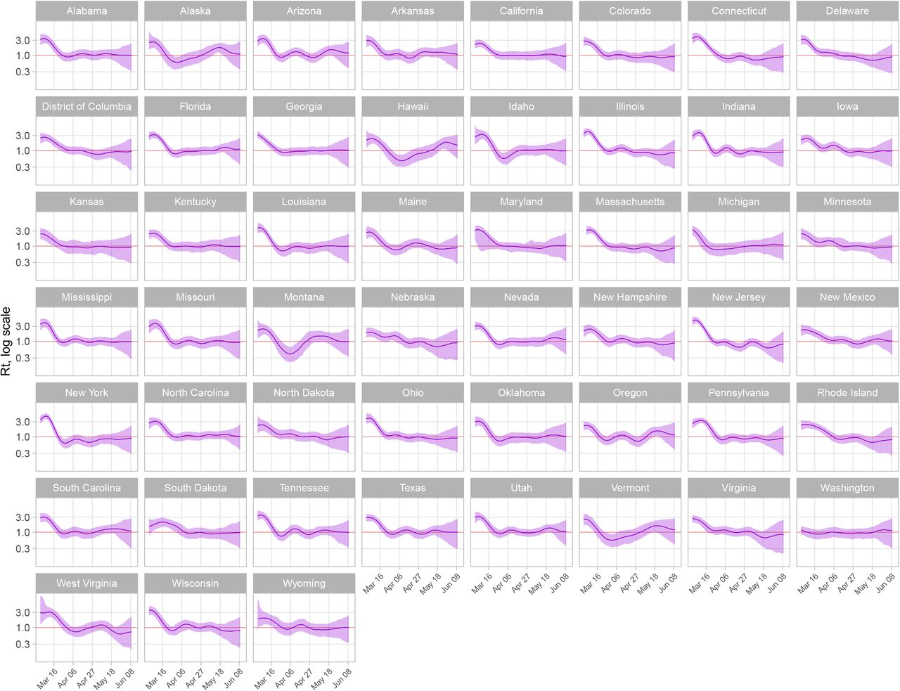
Effective reproduction number (Rt) estimates by state, log scale. Estimates from March 1 to June 11, 2020 are shown.
We compare our estimates of COVID-19 incident deaths (detected and undetected) to estimates of excess all-cause mortality (2) (Fig. 4). We present comparisons to states where all-cause mortality was higher at each weekly timepoint from March 21 – May 9 than the expected number of deaths (based on all-cause mortality from 2015 – 2019). We expect COVID-19 deaths to follow similar trajectories to, but be less than, estimated all-cause mortality, which will include additional non-COVID-19 deaths linked to the social disruption caused by the pandemic (2). On average, the median modeled estimate of COVID-19 deaths is less than estimates of excess all-cause mortality, though uncertainty bounds around COVID-19 mortality estimates typically include estimates of excess all-cause mortality.

Seroprevalence and cumulative death estimates. Top: seroprevalence estimates (cumulative incident infections divided by state population) for June 11, 2020. Bottom: Comparison of modeled incident deaths, modeled reported deaths, estimated excess all-cause mortality.
Additionally, we estimate cumulative incidence of COVID-19 infections as of June 11, 2020 (Fig. 4), as well as at each time point since the beginning of the epidemic. Ideally, these estimates would be compared with population-representative seroprevalence studies, although few state-wide serosurveys have yet been completed. We estimate seroprevalence in New York State to be 10.8% (5.55%, 24.3%) on April 19 and 11.3% (5.78%, 25.3%) on April 28. A recent seroprevalence survey (5) suggested New York State’s seroprevalence in that period was 14.0% (95% confidence interval: 13.3%, 14.7%). Serosurvey estimates are dependent on test characteristics such as sensitivity and specificity, which are not precisely known, as well as an unbiased representative population sample; the authors report possible alternative seroprevalence estimates of 9.8% (9.1% - 10.5%) and 15.0% (14.3%, 15.7%).
As a sensitivity analysis, we ran the model in Delaware, Iowa, and New Jersey without adjustments for secular changes in case and death ascertainment over the course of the epidemic. We chose these states because they had highly variable reported fraction positive, which we used to estimate the completeness of ascertainment (Fig. S3). Removing this adjustment had a small effect on estimates of new infections and Rt, particularly early in the time series when the fraction of positive tests was most unstable (Fig. S4). Additionally, for the main analysis we estimated outcomes using time-series of cases and deaths indexed by date of report. However, some state departments of health have made detailed COVID-19 data publicly available which provide better information on the timing of events. For example, the Massachusetts Department of Public Health regularly publishes daily case counts by date of symptom onset or test and daily death counts by date of death (6). With minor adjustments to the model (described in Materials and Methods), we produced model estimates based on these data. Data type did not noticeably change fit to data and had a small impact on estimates of incident infections and Rt (Fig. S5).
Our approach makes a number of simplifying assumptions related to delays in disease progression and detection. We assume that sojourn time in each health state follows a fixed distribution, and that diagnostic and reporting delays are constant over the course of the epidemic, although we allow for secular changes in the probability that a symptomatic case will be diagnosed. The model is parameterized to estimate only one geographic unit at a time, and we do not model spatial spread of the disease between states. We also make the simplifying assumption that case detection is limited to individuals who are currently symptomatic. This assumption will not hold in situations in which PCR and antibody test results are reported in aggregate or if many asymptomatic individuals are tested for infection, which may lead to biased estimates of COVID-19 case detection. As of June 1, 2020, Arizona and Florida are reporting PCR and antibody tests in aggregate; these test results have previously been reported in aggregate in Iowa, Maine, Michigan, Mississippi, Missouri, New Hampshire, Texas, Virginia, and West Virginia. To date, antibody tests have constituted a small fraction of all reported tests, and so biases in our state-level estimates will be minimal.
We used publicly available data from the COVID Tracking Project (7) to produce the estimates reported here. Because states report cases and deaths in different ways, there are a number of potential inconsistencies in these data. Confirmed and probable cases are reported in aggregate in Idaho, Kansas, and Wyoming as of June 1, 2020, leading to potential upward bias in our estimates of new infections and seroprevalence in these states. Tests are reported as the total number of specimens tested (rather than the total number of individuals tested) in Arizona, California, Connecticut, Georgia, Idaho, Illinois, Maine, Massachusetts, Michigan, Mississippi, New Jersey, Oklahoma, South Carolina, Texas, Virginia, and Wyoming as of June 1, 2020. Our estimates of the probability of diagnosis conditional on symptoms may be upwardly biased in these states, though the size of this bias is likely to be small. Finally, data are subject to occasional audits and revisions. Revisions to cumulative counts of cases and deaths have frequently been implemented as a single-day change in the cumulative count, without matching revisions to the historical time series. This leads to additional variance in the reported data, and a reduction in the precision of reported estimates.
As compared to other approaches for estimating Rt and COVID-19 epidemiological outcomes for US states (8,9) and other countries (10), our approach allows for time-trends in diagnostic coverage, which in turn accounts for under-ascertainment of cases and deaths over the course of the epidemic. Our approach utilizes information on the time-course of the natural history of infection and known lags in reporting systems, in combination with a metric that adjusts for changes in diagnostic test availability, to produce Rt estimates. This provides a coherent framework for simultaneously estimating the trend in disease incidence and the fraction of the population that has already been infected, providing key information on the current status and past severity of state-wide epidemics. These methods can also be applied to more local (e.g., county-level) data to produce a more refined understanding of local epidemics. To that end, we have open-sourced and documented our covidestim R package on GitHub, so that others can easily apply these methods to their own data.
Data Availability
All data used in the main analysis are available from The Covid Tracking Project. Data from Massachusetts used in the sensitivity analysis are available from the Massachusetts Department of Public Health. The covidestim package is available for download.
https://www.mass.gov/info-details/covid-19-response-reporting
Funding
National Institutes of HealthT32 GM007205
National Institute of Allergy and Infectious Diseases R01 AI112970
National Institute of Allergy and Infectious Diseases R01 AI137093
National Institute of Allergy and Infectious Diseases R01 AI146555
National Institute of Allergy and Infectious Diseases R01 AI112438
Fogarty International Center D43 TW010540
Author contributions
TC and NAM conceived the project; MHC and NAM developed the methodology; MR designed the software; KG and JH curated data; MHC and MR visualized results; MHC, TC, NAM, VEP, JLW, DMW contributed to the analysis; MHC prepared the original manuscript draft; all authors contributed to reviewing and editing.
Competing interests
DMW has received consulting fees from Pfizer, Merck, GSK, and Affinivax for topics unrelated to this manuscript and is Principal Investigator on a research grant from Pfizer on an unrelated topic. VEP has received reimbursement from Merck and Pfizer for travel expenses to Scientific Input Engagements unrelated to the topic of this manuscript.
Data and materials availability
All data used in the main analysis are available from The Covid Tracking Project at https://covidtracking.com/. Data from Massachusetts used in the sensitivity analysis are available at https://www.mass.gov/info-details/covid-19-response-reporting. The covidestim package is available for download at https://github.com/covidestim/covidestim.
Acknowledgments
We thank Jeffery Eaton for his thoughts on statistical analysis.
Footnotes
↵‡ These authors share senior authorship


