
ABSTRACT
For an emergent disease, such as Covid-19, with no past epidemiological data to guide models, modelers struggle to make predictions of the course of the epidemic (Cyranoski, Nature News 18 February 2020). The wildly varying predictions make it difficult to base policy decisions on. On the other hand much empirical information is already contained in data of evolving epidemiological profiles. We offer an additional tool, based on general theoretical principles and validated with data, for tracking the turning points, peak and accumulated case numbers of infected and recovered for an epidemic, and to predict its course. Ability to predict the turning points and the epidemic’s end is of crucial importance for fighting the epidemic and planning for a return to normalcy. The accuracy of the prediction of the peaks of the epidemic is validated using data in different regions in China showing the effects of different levels of quarantine. The validated tool can be applied to other countries where Covid-19 has spread, and generally to future epidemics. US is found to have the largest net infection rate, and is predicted to have the largest total infected cases (708K) and will take two weeks longer than Wuhan to reach its turning point, and one week longer than Italy and Germany.
SIGNIFICANCE We offer a practical tool for tracking and predicting the course of an epidemic using the daily data on the infection and recovery. This data-driven tool can predict the turning points two weeks in advance, with an accuracy of 2-3 days, validated using data from various regions in China selected to show the effects of quarantine. It also gives information on how rapid the rise and fall of the case numbers are, and what the peak and total number of infected are. Although empirical, this approach has a sound theoretical foundation; the main components of the results are validated after the epidemic is near an end, as is the case for China, and therefore is generally applicable to future epidemics.
1. Introduction
The current COVID-19 epidemic is caused by a novel corona virus, designated officially as SARS-CoV-2, spreading from Wuhan, the capital city of Hubei province in China (2-4). The new virus seems to have characteristics different from SARS (severe acute respiratory syndrome) (5, 6): it is less deadly but spreads more widely (7-10). Modeling the epidemic as it develops has been difficult (1). Depending on the model assumptions, predictions of when it “turns a corner” for China varies greatly (11-21), up to after 650 million people have been infected before peaking; many have now been shown to be inaccurate (22). Now as the epidemic has subsided in China and become a global pandemic (23, 24), a reliable forecast of the course of the outbreak in each region is critical for the management and containment of the epidemic, and for balancing the impact from the public health crisis vs the economic crisis. China has instituted some of the strictest quarantine measures around Wuhan and Hubei, which may or may not be adoptable in other countries (25-27). It would be useful to extract the dependence of the epidemic’s evolution on the degree of quarantine to guide policy decisions, while also to characterize properties of Covid-19 that are applicable to other countries.
Mainstream epidemiological models have their origin in the SIR (Susceptible, Infected, and Recovered or Removed) model (28) and its many variations. We explain in the Supplementary Information why existing model predictions vary so widely by commenting on the assumptions underlying these models.
These SIR-type models, however, serves a critical purpose for long-range policy planning, such as warning policy-decision makers of the gravity of the potential impact and prompting them to take proper actions before it is too late. After the breakout, more information is needed for more detailed planning, such as the arrival of the critical turning points, the number of hospital bed we might need at the peak, and the estimate for when to lift the quarantine, and when to return to normalcy. We offer here an additional tool that has the advantage that it has does not depend on the elusive infection rate or the susceptible population, information needed for most models, but has the disadvantage that it cannot be used when the epidemic first started and the data are inaccurate or incomplete. It is based on daily case numbers (i.e. newly confirmed cases), N(t), and recovered cases, R(t).
Without universal testing, the confirmed case number might be only a subset of the true total infected number, which may never be known unless frequent universal testing is instituted. The asymptomatic infected who are not tested and then recover on their own do not get counted but they also do not tax hospital resources. Nevertheless, they can infect others and some of the latter may develop more serious symptoms that require hospitalization. Then these secondary infections are included in our case data. Our aim is to provide a tool that can be used for the management of medical resources. Since we do not use a model to calculate how the asymptomatic infectives infect others, we do not need to know either the infection rate or the asymptomatic infective numbers. Since those who are admitted to the hospital either recover after a hospital stay of T days, or dead after a similar number of days, there should be a delayed relationship between N(t) and R(t), which we will explore in the Theory section. Now that the epidemic in China appears to have come to an end, the data from various regions in China can be used to validate the model. After validation we then apply it to other regions in the world.
Our estimate of the end date of the epidemic is not based on the number of susceptibles, S, approaching zero as in most models (i.e. most of the population is infected, hence acquiring immunity), but N(t) approaching zero and remaining so for two incubation periods. The first incubation period is to allow the asymptomatic infected to show symptoms and the second period to allow those that are infected by the asymptomatic infected to show symptoms. For prediction purpose, the date when the N(t) is zero is estimated by 3 standard deviations from its peak. These two quantities can be extracted from the data as the epidemic is developing. Our estimate of the end of the epidemic is earlier than most model predictions, usually significantly so, because it does not depend on the herd immunity concept.
As is true for all data-driven approaches, our result inevitably depends on the quality of the data used, and some of the early data of the epidemic are not as good as the later data, when better diagnostic methods and more complete reporting are established. However, many of the metrics commonly in use require accumulation of data from the beginning of the epidemic, and consequently are affected by poor data or change of diagnostic methods along the way. We try to avoid accumulation and use local-in-time metrics. Nevertheless, data problems cannot be avoided.
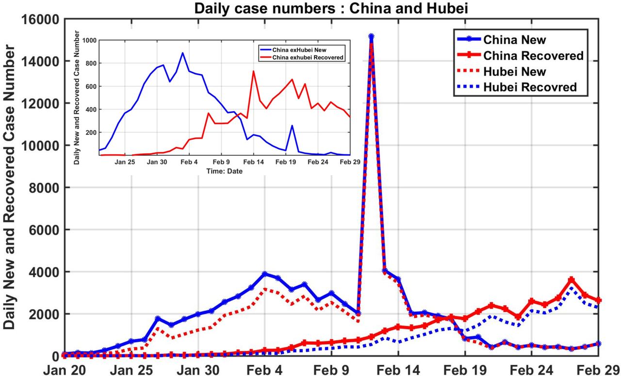
Sensitivity of our conclusion on data problems is extensively discussed in this work. Figure S1 displays examples of data used in this study. One problem immediately becomes obvious for the Chinese data: On 12 February, when Hubei changed its definition of confirmed infection from the gold standard of nucleic acid gene-sequencing tests to clinical observations and radiological chest scans, over 14,000 newly infected cases were added that day, creating a peak that has not been exceeded since. Overwhelmed doctors in Wuhan pleaded for the change so that they did not have to wait for the returned tests to confirm the infection. Outside Hubei, there was no change in definition for the “infected”. How this artifact affects our conclusion will be discussed.
2. Model and its validation using data
Definition: Let I(t) be the number of active infected at time t. Its change is given by;
 where N(t) is the number of newly infected, and R(t), designated as removed, is the sum of the daily recovered and dead. For a disease such as Covid-19 with low fatality rate, R(t) consists of mainly recovered. However even for this disease, the fatality rate in some regions, such as in Northern Italy, approaches 10%. For these regions R(t) should include the dead as well. Note that for the theory part, N(t) includes both confirmed and unconfirmed cases. The term: Existing Infected Case (EIC) number is used to denote the confirmed I(t) when we deal with data.
Let tp, the turning point defined as the peak of the active infected number. At this point maximum medical resource is needed. This maximum occurs when  , implying N(tp) = R(tp).
This is a local-in-time metric. There is therefore no need to first find I(t) to locate this peak. After the turning point, the newly recovered starts to exceed the newly infected. The demand for medical resources, such as hospital beds, isolation wards and respirators, starts to decrease.
The theoretical foundation for our model is given in Supplementary Information. Here we discuss the main results and offer validation of these results using data from China.
Main Result
The daily newly recovered/removed number R(t), is related to the daily newly infected number N(t) as:
 for t>T, where T is the mean recovery period.
This result can be rigorously derived using an age-structured population model (see reference (36)). It is also common sense: the infected eventually recovered after a number of days, or dead after a similar number of days. Of course, the number of days a patient stays in the hospital before discharge depends on the efficacy of treatment and so varies somewhat, and the time it takes for a patient to die may also depend on the age and underlying conditions. T is therefore a statistical quantity.
Validation
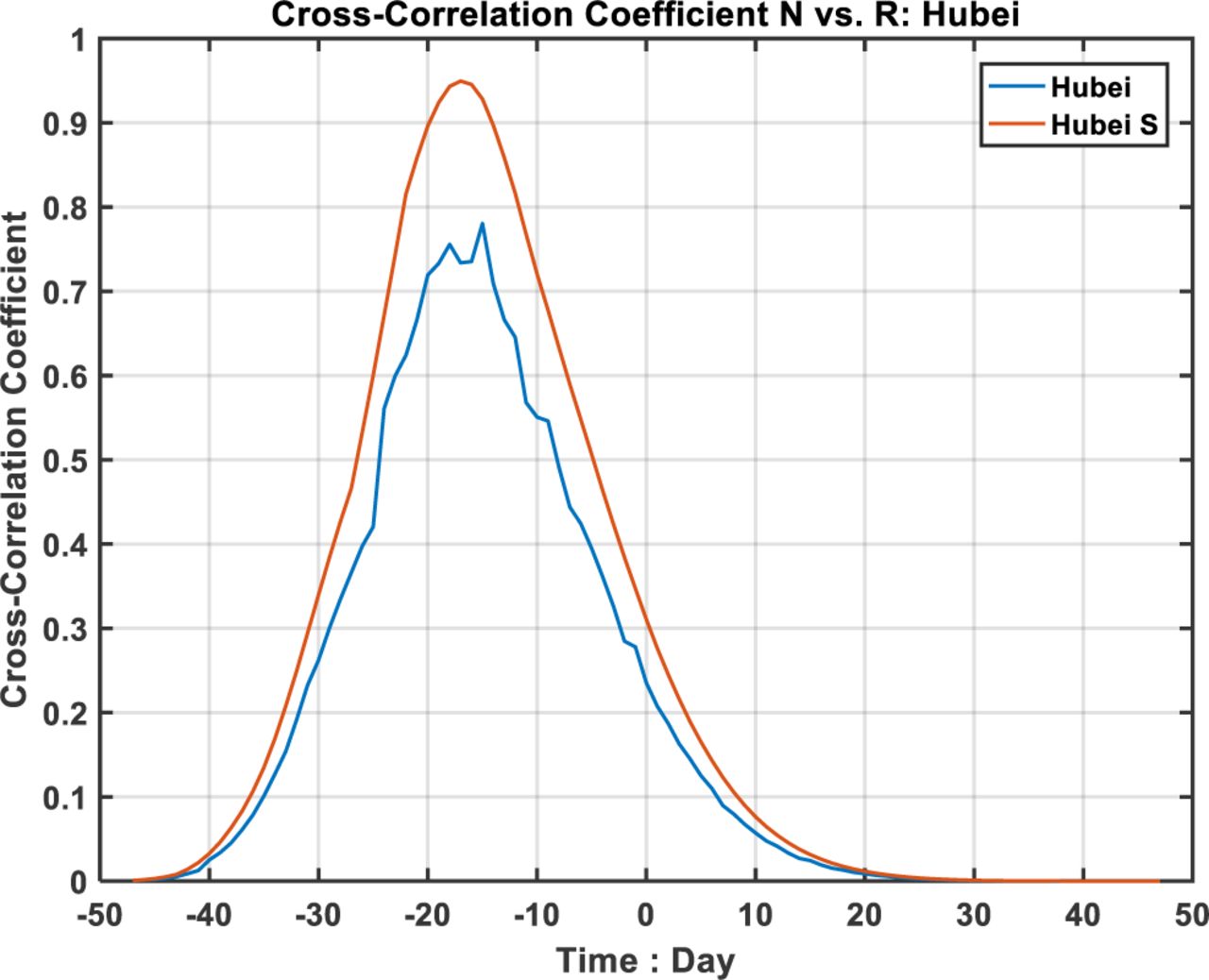
This fundamental relationship can be validated statistically with data. Figures 1, obtained using data from China during the Covid-19 epidemic, shows that N(t) and R(t) are highly correlated: with correlation coefficient of 0.95 when both distributions are smoothed with 5-point boxcar. The unsmoothed daily data also yield a high correlation coefficient of 0.80, with R(t) lagging N(t) by T∼15 days. Both correlation coefficients are statistically significant. A similar result is found for Hubei (Figure S2) and other regions (not shown). This is one of the ways the mean recovery period is determined statistically from data, but it is not practical in the early phase of the epidemic. We will give different methods for the latter purpose. The result on T is consistent with that estimated or predicted later using the slope of the distribution in Figure 4. The latter, obtained by the intercept of the straight line, is less accurate because of the slope is rather shallow.

Lagged correlation of case numbers R(t) and N(t) for China as a whole.
Main Result
The natural logarithm of the ratio of N and R is a linear function of time for t > T. This relationship is important for the purpose of forecast because it is easy to extrapolate from a straight line into the future.
Validation of log NR as a straight line
From data we use the report newly confirmed case number and the recovered case number to define NR ratio as
At tp, NR=1.
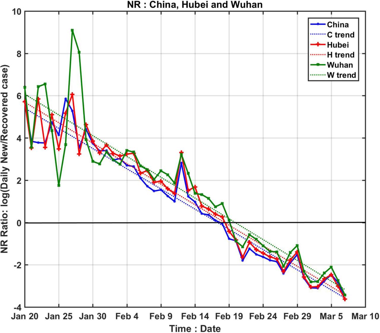
We show in Figure 2, using the data of the epidemic for COVID-19, that the logarithm of NR(t) lies on a straight line, with small scatter, passing through the turning point tp. And data for various stages of the epidemic, from the initial exponential growth stage, to near the peak of EIC, and then past the peak, all lie on the same straight line. The intercept with logNR=0 yields the turning point. This line, obtained by linear-least-square fit in the semi-log plot, is little affected by the rather large artificial spike in the data on 12 February because of its short duration and the logarithmic value. That reporting problem is necessarily of short duration because, on the date of definition change, previous week’s cases of infected according to the new criteria were reported in one day. After that, the book is cleared, and N(t) returned to its normal range.

Logarithm of the ratio of daily newly infected to newly recovered. They lie on straight lines with some small scatter. The dotted straight lines are obtained by linear-least squares fit is. The slopes of the lines are almost the same but with different intercept; the trend lines cross zero (the black solid line) at different time for different regions indicating different peaking time for EIC. The epicenter Wuhan (green) has latest turning point than its province Hubei (pink), which has a later turning point than China as a whole (cyan).
The theoretical result in SI suggests that the slope of the linear line is -T/ σR2, where σR is the standard deviation of the R(t) profile. In general, the slope can be different for different regions with different levels of quarantine and epidemic characteristics. The hospital treatment efficacy would influence T directly. The effect of quarantine would influence the value of σN, the standard deviation of the newly infected, and so indirectly R(t) and σR. Our empirical result from Fig. 2 however shows that the slope is the almost the same for different regions in China, implying that efficacy of treatment and level of quarantine affect T and σ2 proportionally.
Result
The derivative of log N(t) and of log R(t) is each a linear function of time, with known slope. Their intercept with the zero derivative line yields the time for their respective peak.
Validation
Empirically, the derivative of log N(t) or log R(t) lies on a straight line, as shown in Fig. 3 (although the scatter is larger as to be expected for any differentiation of empirical data). The positive and negative outliers one day before and after 12 Feb are caused by the spike up and then down, with little effect on the fitted linear trend (but increases its variance and therefore uncertainty). Moreover, the straight line extends without appreciable change in slope beyond the peak of N(t), suggesting that the distribution of the newly infected number is approximately Gaussian. The mean recovery time T can be predicted as tR − tN, where tR is the peak of R(t) and tN is the peak of N(t). These two peak times can be obtained by extending the straight line in Fig. 3 to intersect the zero line. This predicted result can be verified statistically after the fact by the lagged correlation of R(t) and N(t). If the distribution is indeed Gaussian or even approximately so, the slope in Fig. 3 would be proportional to the reciprocal of the square of its standard deviation, σ, as (See SI):


The derivative of the logarithm of daily newly infected or recovered. Notice the clear separation of the new and recovered cases and also the subtle difference of their slopes. The zero crossings of the trend line give the peak dates of the new and recovered case respectively. And the slopes give an estimate of σ values. In this Figure, the following abbreviations are used: C=China; H=Hubei; N=New Case; R=Recovered.
Similarly result holds for the daily number of recovered, R(t).
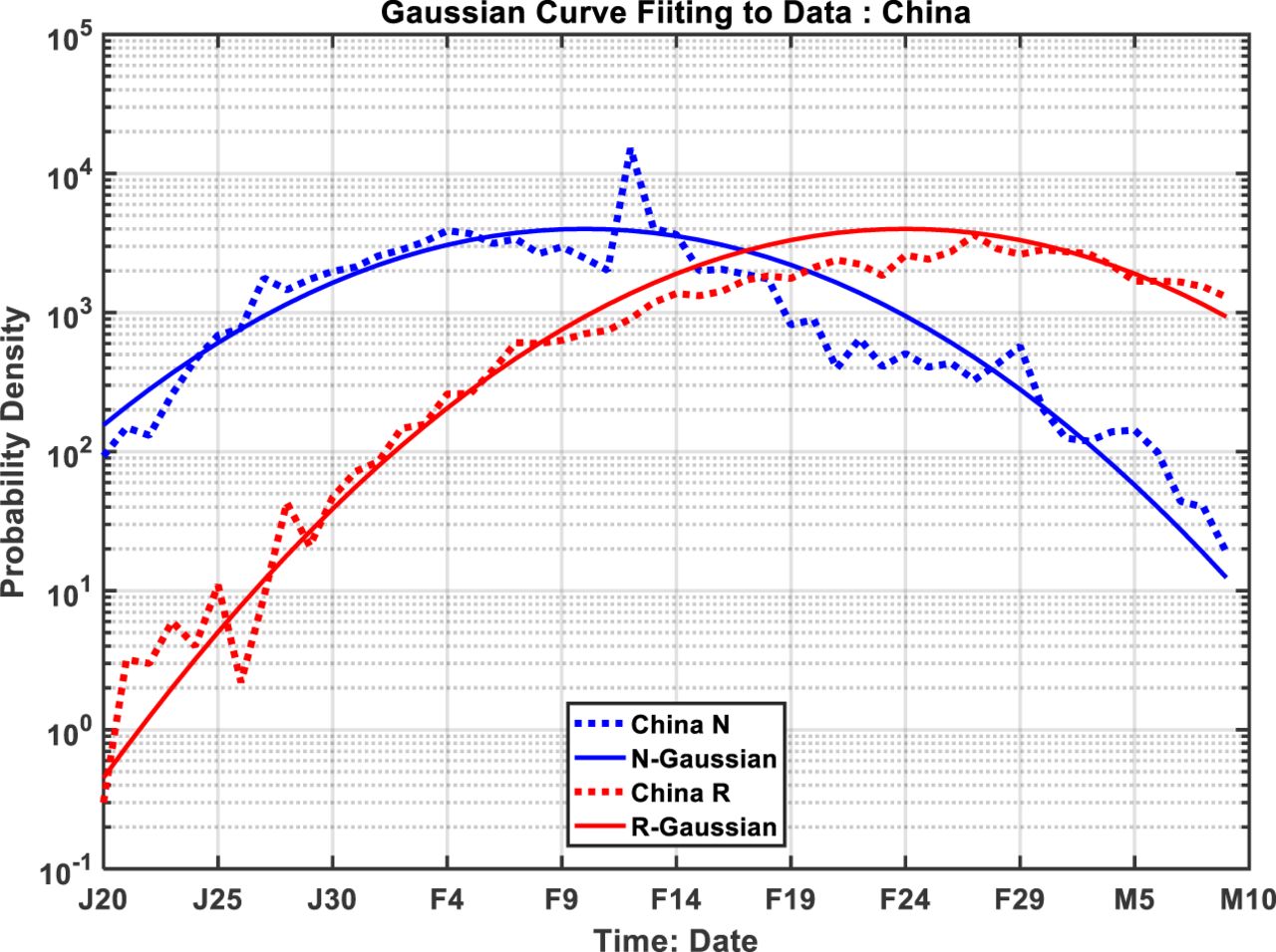
After the epidemic is nearing the end as is the case in China, fitting the data to a Gaussian can be done after the fact (see Figures S3 and S4). The fit is satisfactory even without using any disposal parameters. The parameters used are determined using slopes of log N and log R (see Table S1)
The inferred statistical characteristics of the Covid-19 epidemic are summarized in Table S1 for various regions. The mean recovery time T, is about 13 days for China as a whole. For Wuhan, the city at the epicenter whose hospitals were more overwhelmed and the patients admitted into hospitals more seriously ill than those in other provinces, T ∼16 days, while that for Hubei is 14 days. The standard deviation, σ, is found to be around 8 days, with slight difference between that for N(t) and for R(t), with one exception for Hubei outside Wuhan. Such a fine subdivision may not be practical for the data quality we have. The σ tends to be smaller for China as a whole than Wuhan. One can see that T and σ2 indeed varying approximately in proportion.
The peak infected cases
Writing  , and noting
  , the exponent is
  . Hence the peak infected case number can be predicted, using the predicted value for tN starting from a conveniently chosen time tB, such as the latest time with data available, as:

Accumulated quantities
To calculate I(t) using reported data, only confirmed cases are used (We call it EIC). It is given by the accumulated newly confirmed cases minus the accumulated confirmed recovered. Since the accumulation of early poor data can introduce errors a more local-in-time formula is given as:
That is, to find I at time t, one only needs to add up the daily newly infected case numbers for a period of T preceding t. This is an almost local-in-time property even for this accumulated quantity. For validation, we estimate the peak of the I case number on 18 February by computing the sum of daily newly infected case numbers for 15 days, from February 4 to February 18, which yields a peak value for the total infected cases on 18 February of 54,747. This is within 10% of the reported number of 57, 805, even after taking into account the deaths (by subtracting the accumulated deaths of 2,004 from our estimate).
3. Predictability
Prediction of the turning point using NR ratio
We first discuss how the true turning point can be determined from data after it has occurred. Then we give a method for predicting this true value in advance and assess the accuracy of the forecasts as function of days in advance when the prediction is made. A note: after this manuscript was submitted for review the predictions that we made previously have come to pass. Although consequently the value of our predictions has greatly diminished, it gives us a chance to compare our predictions against the truths. This model validation process is important if we are to apply the same method for prediction to other regions.
The turning point and the end of the epidemic are the two most watched markers on its development (28, 29), along with the number of infected at each stage of the epidemic. There are various definitions of the turning point. A common one defines the turning point of the epidemic as the reported daily number of newly infected reaching a peak and then declining. This is the one touted in the various news announcements, and also used by some research groups (22). The fact that the number of newly infected reaching a peak and then declining does not necessarily imply that the epidemic has “turned a corner”, because the total number of active infected can still be rising with the associated urgent need for additional medical resources, such as hospital beds, isolation wards and ventilators. Furthermore, locating this peak is highly susceptible to data glitches and change in diagnostic definition. A more meaningful turning point should be based on the number of confirmed infected individuals, designated as EIC)(15), reaching a peak and then starting to decline. EIC is in theory obtainable from data of the daily number of new confirmed cases, N(t), and the daily number of newly recovered, R(t), by subtracting the accumulated sum of R(t) from the accumulated sum of N(t). Analysis of this accumulated quantity is sensitively affected by accumulation of poorer early data of reported cases, including under-reporting and under-detection of the number of infected caused by insufficient test kits, in addition to the history of changing diagnostic criteria. Moreover in practice its peak is often not detected until several weeks after it has occurred.
Since the maximum of EIC, can be located by the zero of its derivative, we propose using a local-in-time metric of N(tp)=R(tp) at the peak of EIC, tp.
Referring to Figure S1, for China as whole, tp is found to be February 18; for Hubei, the province of the epicenter Wuhan, tp is found to be 19 February, and for China outside Hubei (China exHubei), 12 February, coincidentally on the same day as the Hubei data spike. However there is no such bump in the data outside Hubei, and so is not likely the result of the data artifact. These results, even including that for Hubei, are not affected by the historical data problems because of our local-in-time method for determining the turning point.
Can such a turning point be predicted before it happened, and if so by how many days in advance? Since the logarithm of NR lies on a straight line passing through the turning point of EIC, it would be interesting to explore if the turning point can be predicted by extrapolation using data weeks before it happened by extrapolation along the straight line (see Figure S5). How far in advance this can be done appears to be limited by the poor quality of the initial data. Fig. 4 shows the results of such predictions. The horizontal axis indicates the last date of the data used in the prediction. The beginning date of the data used is 24 January for all experiments. Prior to that day, data quality was poor and the newly recovered number was zero in some days, giving an infinite NR ratio.
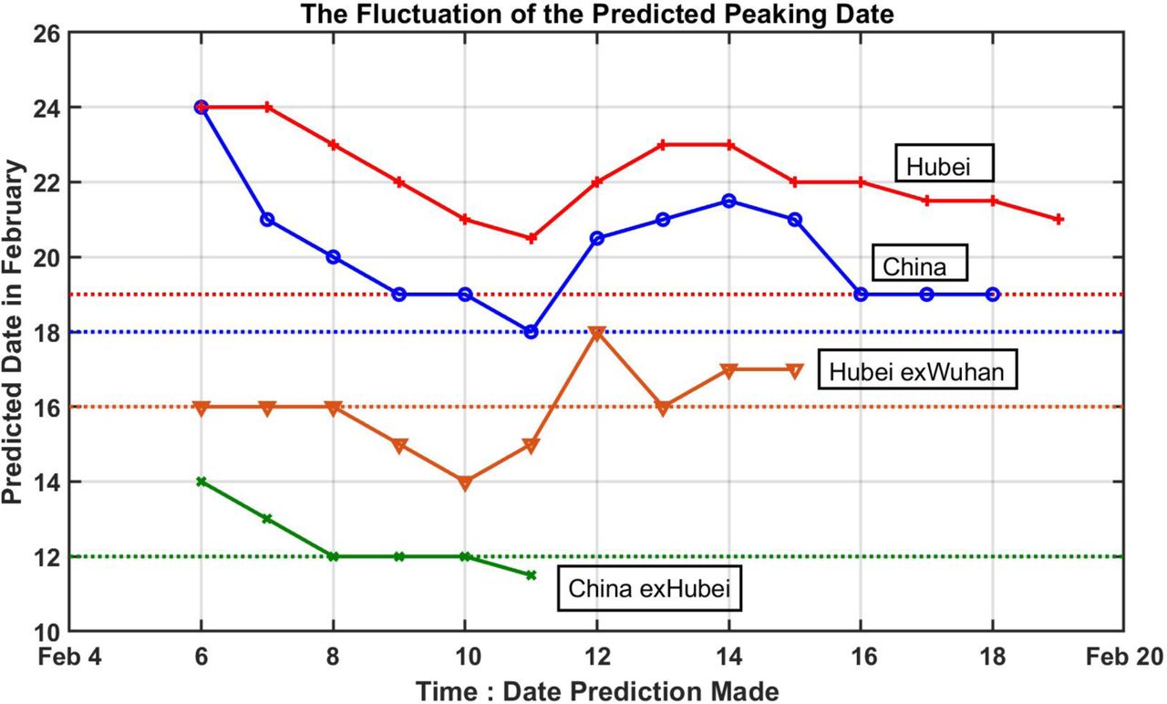
Prediction of the turning point in EIC by extrapolating the trend in logarithm of NR. The horizontal axis indicates the date the prediction is made using data prior to that date. The vertical axis gives the dates of the predicted turning point. Dashed horizontal lines indicated the true dates for the turning point, as determined from Fig. S1.
For China outside Hubei, the prediction made on 6 February gives the turning point as 14 February, two days later than the truth. A prediction made on 8 February already converged to the truth of 12 February, and stays near the truth, differing by no more than fractions of a day with more data.
The huge data glitch on 12 February in Hubei affected the prediction for Hubei, for China as whole, and for Hubei-exWuhan. These three curves all show a bump up starting 12 February, as the slope of N(t) is artificially lifted. Ironically, predictions made earlier than 12 February are actually better. For example, for China as a whole, predictions made on 9 February and 10 February both give 19 February as the turning point, only one day off the truth of 18 February. A prediction made on 11 February actually gives the correct turning point that would occur one week later. At the time these predictions are made, the newly infected cases were rising rapidly, by over 2,000 each day, and later by over 14,000. It would have been incredulous if one were to announce at that time that the epidemic would turn the corner a week later.
Even with the huge spike for the regions affected by the Hubei’s changing of diagnosis criteria, because of its short duration the artifact affects the predicted value by no more than 3 days, and the prediction accuracy soon recovers for China as a whole. For Hubei, the prediction never converges to the true value, but the over-prediction is only 2 days. This smallness of the error is remarkable given that other model predictions differ by weeks or months.
Table S2 lists the mean and standard deviation of the predictions. For applications to other countries and to future epidemics without a change in the definition of the “infection” to such a large extent, we expect even better prediction accuracy.
Estimate of “all clear” declaration
We can now estimate a time for a declaration of “all clear”. No verification is yet possible as the predicted date has not occurred. At the turning point, the EIC is still at its peak. For the disease to have run its course, and an “all clear” declaration can be announced, we require that the newly infected case number to drop to zero. For prediction practice this “zero” is measured by three standard deviations from the peak of N(t). Then we wait for two incubation periods, each 14 days, to pass, before we declare “all clear”. Using the inferred disease characteristics in Table S1, our prediction is, for China outside Hubei: the last week of March. For China as a whole: the first week of April, barring “imports” of infected from abroad. At this point there may still be some patients in the hospital who are infected with the virus. The “all clear” call assumes that these patients are not roaming freely to cause new infections.
Prediction for South Korea
Figure S6 summarized the available data for Korea at the present. The recovered case numbers hovered around 1 and 2 daily up to March 1st. It only picked up toward the end. Starting from 19 February, there seems to be enough new daily infected cases. The South Korea Government has identified that the epic center of the epidemic was at church gatherings in the city of Daegu and North Gyeongsang province, where 90% of the cases are found. Specifically, a confirmed COVID-19 patient was reported to have attend the Shincheonji Church of Jesus services twice on February 9th and 16th. Given the incubation period of 7 to 14 days, the initial explosion at February 19th and the first peak value around February 24th are not accidents.
If we use the available daily new cases data, we can get the statistical characteristics of the distribution of the daily new cases from Figure S7, which gives the tN as March 3rd and a σ N value of 4.5 days. If we further use the turning point as approximately tN+T/2, then the turning point should fall on March 10, assuming T as 14 days based on the over all mean from different regions in China.
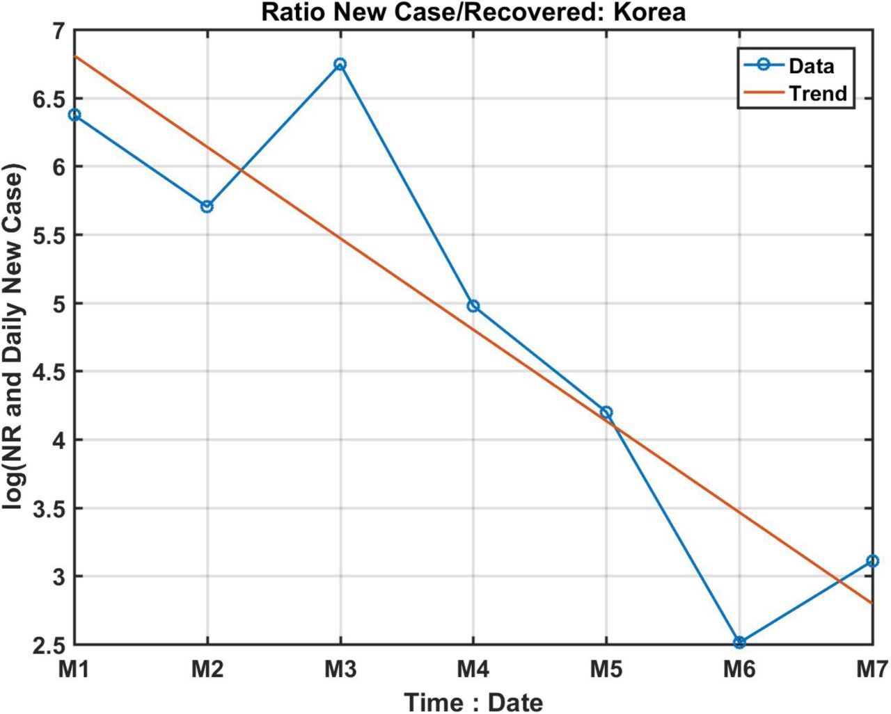
For the NR ratio, it is limited by the availability of recovered case number. If we use the limited recovered cases starting from March 1st, we have 7 days of data. The computed the NR ratio together with the trend is given in Figure S8. The turning point, at the zero-crossing of the extended trend line, would occur between March 11th and 12th. This approach does not need to use a value for T.
An estimate of the end of the epidemic can be given as the second week of April, using the estimated value for tN= 3 March, σ=4.5 days. Remarkably, this date is around the same time as for Wuhan, China. South Korea owes its quick turning point and end of the epidemic date to its ability to identity the first infection and the secondary infections at Shincheonji Church (31), where most of the infected were concentrated. This is reflected in the data: σ for South Korea is only half that of China, with a more rapid rise and fall of the newly infected. Its data for the newly infected are probably more accurate compared to other countries in similar stage of the epidemic, due to its massive and speedy (within 6 hours) testing of the population in its “trace, test and treat” policy.
4. Effects of quarantine judging from data on the net infection rate
Following (15), we define a time-dependent net infection rate as:
In traditional models, such as the SIR model, there is also a time-dependent infection rate, which at t=0 is related to the Basic Reproductive Number R0. If this number is greater than 1 then an epidemic will ensue, i.e. the infected population will increase exponentially after the introduction to a susceptible population S at t=0 some initial infected. That is, from the SIR model equation:
 where aS(t) is the infection rate and b = 1/T is the mean recovery rate.
Therefore  . α(0) = b(R0− 1), with
  .
.
Our time-dependent net infection rate generalizes this concept to be independent of the SIR or other models and be applicable at later times as well: If in the course of an epidemic, α(t) is positive, the number of infected will grow exponentially, reaching a peak number of infected when α(t) = 0 at t = tp. Then the total number of active infected will decrease exponentially. One could in analogy to R0, define a time-dependent Reproductive Number Rt = α(t)T − 1, so that if this number is greater (less) than 1 the number of infected will grow (decrease) at time t. We will here use α(t) directly.
Since α(t) has a zero and its first derivative near the zero is nonzero (viz negative) because tp is the maximum of I(t), it is a linear function of t with negative slope in that neighborhood. This expectation is verified empirically, using data for the total existing case numbers. We find that this time dependent infection rate is approximately a linear function of time in the neighborhood of its zero over a period of a few weeks.
This gives another way to predict the turning point tp which can be used instead of (but is less accurate than) the NR ratio, during the early stage of the epidemic when not enough R(t) data is available, as is the case currently for US.
The peak EIC number can be predicted as
 , where tB is the last available data before the turning point. It is assumed that α(t) lies on a straight line between tB and tp.
Predicting the peak active infected cases
Since the turning point can be predicted two weeks in advance, the above formula can be used to predict the peak EIC numbers.
Predicting the total infected cases (TIC)
To predict the total infected cases for the epidemic for a region, we need to do the above accumulation of N(t) into the future, to the end date of the epidemic. That total is approximately:
 assuming that N(t) is approximately symmetric about its peak at tN. In reality N(t) may not be symmetric and likely has a long tail. However, since the number of cases along the tail is small, the above approximation for the total is still good. If the present time tB is before tN, we need a way to predict TIC(tN). Let the total infection rate be defined as:

By extrapolate the total infection rate forward in time we can predict:

USA
tN is predicted to be 2.2 days from today, April 5. Today’s TIC is 308,850. So the predicted total infected cases for the epidemic when it is over is predicted to be 708,750. This is a very large number, nine times larger than that of China, which has a much larger population, but is nevertheless much lower than some other predictions of a few million infected. Its current EIC is 285,000, and is predicted to peak 12 days from now at 547,000. This is the peak demand for hospital beds.
Germany
Germany has good data. Its tN was 2 days ago. On that day its TIC was 85,000. So the total infected cases for the epidemic when it is over is predicted to be 2 times that: 170,000. Its current EIC is 68,248. The peak EIC is 69,627, which will occur two days from now.
Spain
tN occurred on March 31. On that day its TIC was 94,417. The total TIC when the epidemic is over is predicted to be twice that, 188,800. Its peak EIC is predicted to be 84,250, to occur 4 days from now.
UK
Its current TIC is 41,000. Its tN is 7.5 days from now. Calculating its TIC at that time and then doubling it yields a total TIC of 134,000 when the epidemic is over. The peak EIC is predicted to be 83,200, 16 days from now. This is the peak demand for hospital beds. (It should be noted that the recovered case number for UK is unusually low, currently at 209, while the dead is much higher, at 4,900. The data may be doubtful.)
Comments on the effects of quarantine
Additionally the net infection rate reveals the effect of measures taken with social distancing and quarantine. Figure 5 shows the time-dependent net infection rate for each region starting when the newly confirmed cases exceed 100. This way of plotting facilitates comparison of different regions at the same stage of the epidemic. First, China outside Hubei has the lowest time-dependent infection rate after Hubei was lockdown. Germany and Italy have similar exponential growth rate of the net infected case numbers, both higher than even Wuhan, the epicenter in China. More surprisingly, US has the highest exponential net infection rate, higher than Germany and Italy and China. This can be attributed to the fact that US so far does not have a nation-wide shutdown, unlike these other countries. Secondly, China outside Hubei reached its turning point early, in fact 20 days earlier than the epicenter, Wuhan.

The time-dependent net infection rate (in units of 1/day) as a function of time starting on the date (listed in the inset) when the newly confirmed case number exceeds 100 for each region. To obtain the actual calendar date, add the dates on the horizontal axis to the starting date indicated in the inset. The number of confirmed cases on the starting date is listed at the top.
We had previously predicted this, which is qualitatively different than many model predictions, which had the epicenter achieving its turning point 1-2 weeks earlier than China outside Hubei (13). Italy and Germany are predicted to take a week longer to reach their turning point, while US will take another week longer than it will take Germany and Italy.
That Italy would take the same amount of time to reach its turning point as Germany and has approximately the same net infection rate may be due to two reasons: Italy does not test as widely as Germany and so the case numbers represent a smaller portion of the infected. Secondly Germany has the lowest fatality rate while Italy one of the highest. The number of the dead is about the same as the number of cured for Italy. The dead is included in recovered/removed. If it were not included, EIC would have been higher for Italy. Nevertheless, whether dead or cured, the hospital bed is vacated.
5. Conclusion
We offer an additional data-driven approach to track and predict the course of the epidemic. Many parameters characterizing an epidemic can be determined from local-in-time data. Validated by real data, we suggest that our approach could be applied not just to the current Covid-19 epidemic, but also generally to future epidemics. It could also be used as a practical tool for epidemic management decisions such as quarantine institution and medical resource planning and allocations (32-35).
Two results are of special significance for future policy makers. First the turning point for the epidemic in China exHubei occurred a week earlier than that for Wuhan. Second the US will take 2 weeks longer to reach its turning point than even Wuhan. After its lockdown, Wuhan, with a large susceptible population of 11 million, enforced straight social distancing, which is more strict than that adopted in the US.. As a consequence, even with a large pool of potential susceptible, the outbreak could end sooner, as compared to the time it will take US and Europe. For China, the lockdown of Wuhan and Hubei was the reason why the epidemic outside Hubei was under control, and the turning point occurred earlier. In Wuhan, with hospitals facing the number of infected patients far exceeding available hospital beds in the initial period, some infected patients were not adequately isolated. The infected were sent home and caused secondary infections among family members. This might have played a role in delaying the turning point. On the other hand, outside Hubei, hospitals were not as overwhelmed because of the strict quarantine placed on Hubei, which drastically reduced the import of the disease originating from Hubei. The infected were better isolated, reducing further spread, and treated in hospitals, resulting in shorter time to recovery (see Table S1). This is evidence of the effectiveness of the city and province-wide lockdown in “flattening the curve” outside.
The additional and surprising finding that the net infection rates in Italy, Germany and the US are higher than even Wuhan also manifests the effect of the enforcement of lockdown, stay-at-home and strict social distancing policy in Wuhan, which was much stricter than those adopted currently in Europe and US. The more lax latitude and lack of enforcement in the US will lead to a longer period of the epidemic, longer than even Italy, and the largest number of total infected cases of 710,000 before it is over.
Data Availability
All data used in this study are publicly available.
Competing Interests
The authors declare no competing interests.
Data Availability
All data in this study are publicly available from World Health Organization (WHO) at https://www.who.int/emergencies/diseases/novel-coronavirus-2019/situation-reports/ and on the Daily Brief site of the China’s National Health Commission at http://en.nhc.gov.cn/
The Korean data is available at https://sa.sogou.com/new-weball/page/sgs/epidemic Coronavirus COVID-19 Global Cases by Johns Hopkins CSSE https://gisanddata.maps.arcgis.com/apps/opsdashboard/index.html#/bda7594740fd40299423467b48e9ecf6
Supplementary Information
Comments on SIR-type of models
Mainstream epidemiological models have their origin in the SIR (Susceptible, Infected, and Recovered or Removed) model (28) and its many variations. We discuss here why existing model predictions vary so widely by commenting on the assumptions underlying these models, using the classical SIR model as an example.
The number of the infected is increased by the rate of infection, which is assumed to be aIS, and decreased by the rate of recovery/removed, who are assumed to be immune to further infection, bI. (dI / dt = aIS − bI). This latter category, R, increases at the rate of bI. (dR / dt = bI). Both of the parameters, especially the infection rate a, is largely unknown for an emergent disease (1), and have to be either estimated based on limited statistics the number of contacts a single infected person may have and how many of the contacted people will be infected, or obtained by curve fitting of reported I(t). This approach has problems. First, for Covid-19, there is a population of asymptomatic infected, which may be larger than the reported/confirmed I during the early stages of the epidemic, when wide-scale testing is not available. Since this asymptomatic infected is also infectious, and some of those infected by them could later become confirmed infected, fitting the rate of increase of reported I to estimate the infection rate would inevitably yield a much larger a. Consequently the model predictions using this estimated parameter value may yield a very large peak infection number. Secondly, since dI / dt = aI(S − b / a), the number of infected will increase (approximately exponentially) for S > b / a, but for a new virus to which the population has no immunity, the susceptible population could be very large. For China it could be as large as 1.4 billion. For Hubei it is 65 million. The susceptible population should be lower if the quarantine of Wuhan were tight, but it is difficult to estimate what it is under realistic conditions. Thirdly, predictions of the end of the epidemic vary widely because of the basic assumption in some SIR type of models that if most of the population is infected and recovered (and hence acquired immunity) or dead (and hence no longer infectious). The concept of “herd immunity” is rooted in the idea that with enough of the population acquiring immunity this way (or from a vaccine if one is developed in time), the susceptible population is reduced to S < b / a, and the rate of increase of I will turn negative. This will require as much as 70%-90% of the population be infected, a huge number. Modern models take into account of the effect of quarantine and isolation in reducing the number of people each infected can contact, thus reducing the infection rate a, so that S does not have to be reduced to such an extent for the epidemic to peak and I starts to decrease. However, such estimates are very dependent on model assumptions.
Of course the modern models of epidemiology are more sophisticated than the SIR model (12-14, 17, 21).
We offer here an additional tool that has the advantage that it has does not depend on the elusive infection rate or the susceptible population, information needed for most models, but has the disadvantage that it cannot be used when the epidemic first started and the data are inaccurate or incomplete. It is based on daily case numbers (i.e. newly confirmed cases), N(t), and recovered cases, R(t).
Our estimate of the end date of the epidemic is not based on the number of susceptibles, S, approaching zero as in most models (i.e. most of the population is infected, hence acquiring immunity), but N(t) approaching zero and remaining so for two incubation periods. The first incubation period is to allow the asymptomatic infected to show symptoms and the second period to allow those that are infected by the asymptomatic infected to show symptoms. For prediction purpose, the date when the N(t) is zero is estimated by 3 standard deviations from its peak. These two quantities can be extracted from the data as the epidemic is developing. Our estimate of the end of the epidemic is earlier than most model predictions, usually significantly so, because it does not depend on the herd immunity concept.
THEORY
Definition: Let I(t) be the number of active infected at time t. Its change is given by;
 where N(t) is the number of newly infected, and R(t) that of the newly recovered or removed (dead). Note that for the theory part, N(t) includes both confirmed and unconfirmed cases. The term: Existing Infected Case (EIC) number is used to denote the confirmed I(t) when we deal with data.
Let tp, the turning point defined as the peak of the active infected number. At this point maximum medical resource is needed. This maximum occurs when  , implying N(tp) = R(tp).
There is no need to first find I(t) to locate this peak. After the turning point, the newly recovered starts to exceed the newly infected. The demand for medical resources, such as hospital beds, isolation wards and respirators, starts to decrease.
Let t = 0 be when the first infection began. For Wuhan, China, this date is near the end of 2019, perhaps even earlier. Let tB be the beginning of the better quality data. This time is beyond the initial incubation period of the disease and it can be assumed that at that time there is already a population of infected, some of them asymptomatic but nevertheless infectious.
Let X(t,s) be the number of infected cases at time t, with s being the “age” distribution, i.e. number of days sick.
The total number of infected is given by:
After being sick for T days, a patient either recovers or is removed (dead). T is called the recovery period (or removal period). It is also called the infectious time if the patient is infectious during this period. Of course its value varies by patient and by the efficacy of treatment for each hospital. For the removed it also depends on the age of the patient and whether there are underlying medical conditions. Only a mean recovery period is obtainable from data, and so this is in reality a statistical quantity. We will discuss later how this statistical quantity can be obtained from data.
Conservation law (see Murray: Mathematical Biology Part I, Chapter 1 (36)): After first infected and until removed or cured, we have:
So, since ds / dt = 1,

This equation is to be solved using the method of characteristics as
X(t, s) = constant along characteristics defined by ds dt = 1.
Boundary condition: X(t, 0), specifies the “birth” process, i.e. how the disease spawns newly infected (with “age” s = 0).
Initial condition: X(0,s) = 0 for s > 0, specifies the initial age distribution at t = 0
There are two types of characteristics:
The first type of characteristics intersects the t = 0 axis, and since the initial condition is zero, we have the solution:
That is, there is no infected population who is sick for more days than the lapsed time since the first infection occurred.
For the second type of characteristics, t > s the solution is
 with the form of f to be determined by the boundary condition. Even without determining the form of f we have the following general results:
For t > T, and therefore t > s :

Since the rate of increase of confirmed I(t) is by definition equal to the newly confirmed infected number, N(t), minus the newly recovered (or removed) number, R(t), we have:

For a fatal disease with low fatality rate, where almost all infected cases eventually recover after a hospital stay of T days, we can identify
f (t) with N(t), and f (t − T) with R(t).
If the disease has a non-negligible fatality rate, we include the dead in R(t).
Main Result
The daily newly recovered/removed number R(t), is related to the daily newly infected number N(t) as, for t > T :
Validation
This fundamental relationship can be validated statistically with data. Figures 1, obtained using data from China during the Covid-19 epidemic, shows that N(t) and R(t) are highly correlated: with correlation coefficient of 0.95 when both distributions are smoothed with 5-point boxcar. The unsmoothed daily data also yield a high correlation coefficient of 0.80, with R(t) lagging N(t) by T∼15 days. Both correlation coefficients are statistically significant. A similar result is found for Hubei (Figure S2) and other regions (not shown). This is one of the ways the mean recovery period is determined statistically from data, but it is not practical in the early phase of the epidemic. We will give different methods for the latter purpose. The result on T is consistent with that estimated or predicted later using the slope of the distribution in Figure 4. The latter, obtained by the intercept of the straight line, is less accurate because of the slope is rather shallow. For the regions considered in Figure 1, the fatality rate is small and so the dead are not included in R(t) for convenience.
The second type of characteristics intersects the boundary s = 0. The boundary condition itself needs to be solved as a function of t to describe how new infection (at s = 0) occurs. This can be done using a birth model, such as Eq. (1.56) in (36). For our purpose we assume that the solution of this model yields a distribution with age that has a full spectrum 0 < s < T of infectives at a time tB, long after a full incubation period has passed.
 ; A independent of s.

Therefore the solution is, for t > tB > 0:
 where tN is the peak of N(t), and tR = tN + T is the peak of R(t).
Both distributions are Gaussians.
For tB < t < T,

Again, N(t) is Gaussian, but there is no recovered or removed during this early stage.
Main Result
The natural logarithm of the ratio of N and R is a linear function of time for t > T :
 a linear function of t. This relationship is important for the purpose of forecast because it is easy to extrapolate from a straight line into the future.
It intersects 0 at  . This yields the turning point, when the NR ratio is 1, and therefore its logarithm is zero.
Result: The turning point, defined as the maximum of I(t), is given by  .
.
Result: The slope of log NR is equal to 4 /T.
When time is normalized by T, the derivative is given by:
 , a dimensionless constant.
Heterogeneous Data
The above results are obtained for the case of a single introduction into a region of infected at t=0 and we solve for the subsequent development of the epidemic from that single source. Consider now a large region consisting of a number of small regions, and the “seeding” of the infected occurs at different times for different regions. The large region could be China, and the first infection could be Wuhan, Hubei and then the regions outside Hubei. Then we may have for the China as a whole data for the newly infected a sum of several Gaussians staggered in time. As long as the Gaussians are not separated so much that there are different peaks in the combined data, the combined data can still be considered as Gaussian, as is the case in the real data. However, the standard deviation σ of the combined Gaussian is inevitably larger and is no longer given by b:
We still have R(t) = N(t − T) since this result holds for each sub-region. The result that log NR is a linear function of time still holds:
The slope of the straight line is  .
.
Since the hospital state can add as a smoothing filter on N(t) to yield R(t), the standard deviation for R(t) could be slightly wider than that for N(t). So we could have two different Gaussians (but their integral over all time should be the same):
Taking this into account, we have, denoting T = tR − tN :

As the values of σN and σR are very close based on the empirical data, the quadratic term is always small comparing to the other terms for the length of time we are considering here. Hence.
 a linear function of time. Its slope is
  .
.
Result: The natural logarithm of the ratio of two Gaussians of slightly different standard deviation is approximately a straight line.
Validation of log NR as a straight line
From data we use the report newly confirmed case number and the recovered case number to define NR ratio as

At tp, NR=1.
We show in Figure 2, using the data of the epidemic for COVID-19, that the logarithm of NR(t) lies on a straight line, with small scatter, passing through the turning point tp. And data for various stages of the epidemic, from the initial exponential growth stage, to near the peak of EIC, and then past the peak, all lie on the same straight line. The intercept with logNR=0 yields the turning point. This line, obtained by linear-least-square fit in the semi-log plot, is little affected by the rather large artificial spike in the data on 12 February because of its short duration and the logarithmic value. That reporting problem is necessarily of short duration because, on the date of definition change, previous week’s cases of infected according to the new criteria were reported in one day. After that, the book is cleared, and N(t) returned to its normal range.
The theoretical result suggests that the slope of the linear line is -T/ σR2, where σR is the standard deviation of the R(t) profile. In general, the slope can be different for different regions with different levels of quarantine and epidemic characteristics. The hospital treatment efficacy would influence T directly. The effect of quarantine would influence the value of σN, the standard deviation of the newly infected, and so indirectly R(t) and σR. Our empirical result from Fig. 2 however shows that the slope is the almost the same for different regions in China, implying that efficacy of treatment and level of quarantine affect T and σ2 proportionally.
Validation of the slope of log N(t) and log R(t)
Interestingly, the derivative of log N(t) or log R(t) also lies on a straight line, as shown in Fig. 3 (although the scatter is larger as to be expected for any differentiation of empirical data). The positive and negative outliers one day before and after 12 Feb are caused by the spike up and then down, with little effect on the fitted linear trend (but increases its variance and therefore uncertainty). Moreover, the straight line extends without appreciable change in slope beyond the peak of N(t), suggesting that the distribution of the newly infected number is approximately Gaussian. The mean recovery time T can be predicted as tR − tN, where tR is the peak of R(t) and tN is the peak of N(t). These two peak times can be obtained by extending the straight line in Fig. 3 to intersect the zero line. This predicted result can be verified statistically after the fact by the lagged correlation of R(t) and N(t). If the distribution is indeed Gaussian or even approximately so, the slope in Fig. 3 would be proportional to the reciprocal of the square of its standard deviation, σ, as:
Similarly result holds for the daily number of recovered, R(t).
After the epidemic is nearing the end as is the case in China, fitting the data to a Gaussian can be done after the fact (see Figures S3 and S4). The fit is satisfactory even without using any disposal parameters. The parameters used are determined using slopes of log N and log R (see Table S1)
The inferred statistical characteristics of the Covid-19 epidemic are summarized in Table S1 for various regions. The mean recovery time T, is about 13 days for China as a whole. For Wuhan, the city at the epicenter whose hospitals were more overwhelmed and the patients admitted into hospitals more seriously ill than those in other provinces, T ∼16 days, while that for Hubei is 14 days. The standard deviation, σ, is found to be around 8 days, with slight difference between that for N(t) and for R(t), with one exception for Hubei outside Wuhan. Such a fine subdivision may not be practical for the data quality we have. The σ tends to be smaller for China as a whole than Wuhan. One can see that T and σ2 indeed varying approximately in proportion.

The daily newly infected (in blue) and the daily newly recovered (in red), as a function of time for China as a whole (in solid lines) and Hubei (in dotted lines). The turning point is determined by when the red and blue curves cross. Inset: For China outside Hubei.

Lagged correlation of R(t) with N(t) for Hubei province.

Gaussian fit of N(t) and R(t), for China as a whole.

Gaussian fit of N(t) and R(t), for Hubei Province.
Statistical characteristics of the COVID-19 epidemic in different regions in China inferred from data, for N(t), the daily number of newly infected and for R(t), the daily number of recovered.
Predicted turning point dates. Shown are the mean and standard deviation of the predictions over the prediction period, using the NR ratio method
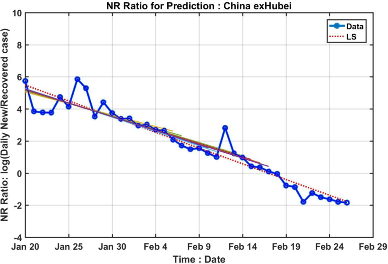
Prediction of the turning point of EIC using linear least-squares trends using various data lengths for China exHubei. All data used start from 24 January. Different colored straight lines show the linear trend calculated from 24 January to a particular date. The spread is over a very small range. Then these trends are extrapolated (extrapolations not shown) to intersect the zero line to yield a prediction for the turning point. The blue dots are the data.

The available data from South Korea (as of March 7th). The sporadic recovered case numbers are mostly in the single digit. If we use the sudden increase of recovered case matching with the sudden explosive increase of new infected, the distance is approximately 14 days, a reasonable T value when compared to the mean value in China. For our data analysis, we used daily newly cases starting February 19th, for the derivative of individual distribution study; we used data case from March 1st, for the NR ratio study, in order to have enough recovered cases.

The derivative of the logarithmic value of daily new infected case distribution.
The NR ratio from 7 days of data from March 1st to 7th. The estimated zero-crossing time would occur between March 11th and 12th, a value consistent with the statistics from the daily new case distribution on March 10th.
Acknowledgements
NEH and FQ are supported by the National Natural Science Foundation of China under Grant 41821004. KKT’s research is supported by the Frederic and Julia Wan Endowed Professorship.
References


