
Abstract
Relevant pandemic-spread scenario simulations provide guiding principles for containment and mitigation policy developments. Here we devise a simple model to predict the effectiveness of different mitigation strategies. The model consists of a set of simple differential equations considering the population size, reported and unreported infections, reported and unreported recoveries and the number of Covid-19-inflicted deaths. For simplification, we assume that Covid-19 survivors are immune (e.g. mutations are not considered) and that the virus can only be passed on by persons with undetected infections. While the latter assumption is a simplification (it is neglected that e.g. hospital staff may be infected by detected patients with symptoms), it was introduced here to keep the model as simple as possible. Moreover, the current version of the model does not account for age-dependent differences in the death rates, but considers higher mortality rates due to temporary shortage of intensive care units. Some of the model parameters have been fitted to the reported cases outside of China1 from January 22 to March 12 of the 2020 Covid-19 pandemic. The other parameters were chosen in a plausible range to the best of our knowledge. We compared infection rates, the total number of people getting infected and the number of deaths in six different scenarios. Social distancing or increased testing can contain or drastically reduce the infections and the predicted number of deaths when compared to a situation without mitigation. We find that mass-testing alone and subsequent isolation of detected cases can be an effective mitigation strategy, alone and in combination with social distancing. However, unless one assumes that the virus can be globally defeated by reducing the number of infected persons to zero, testing must be upheld, albeit at reduced intensity, to prevent sub-sequent waves of infection. The model suggests that testing strategies can be equally effective as social distancing, though at much lower economical costs. We discuss how our mathematical model may help to devise an optimal mix of mitigation strategies against the Covid-19 pandemic. The website corona-lab.ch provides an interactive simulation tool based on the presented model.
Lay Summary The Covid-19 pandemic is a serious threat that can be mitigated by different strategies. Social isolation is currently practiced in most countries in Europe, at least until alternative mitigation strategies can be implemented or therapies and vaccines become available. We have formulated a simple mathematical model to estimate how well social isolation or improved identification of Covid-19 infected people can slow down virus spread and reduce the death toll.
Thereby, we found that improving Covid-19 detection is a highly efficient mitigation strategy. This could be achieved by ramping up testing and following up transmission contacts. These measures can complement and might eventually replace isolation strategies. Testing a random fraction of the susceptible population every day could stop spread of the pandemic. However, unless the virus can be defeated completely and globally, social distancing and/or improved Covid-19 detection must be maintained until therapies or vaccines become available.
1. Introduction
The recent outbreak of Covid-19 in Wuhan, China has led to a pandemic with significant impacts on public-health and economy across the globe. As the number of infected people increases in a community, public health policies move away from containment of the outbreak to mitigation strategies such as social distancing and isolation, with considerable detrimental effects on public life and the economy. While less restrictive mitigation strategies would be desirable, alternative choices are limited due to a lack of resources and technologies. To better understand the potential effects of a particular mitigation strategy, we must assess the underlying factors that impact the spread of the outbreak, and therefore mathematical models integrating the relevant underlying mechanisms are a good tool.
Various bio-mathematical approaches have been proposed and pursued for epidemic-spread modeling. At the highest level one can categorize them into empirical/machine-learning, statistical and dynamical approaches [9]. Yet, due to the lack of sufficient data on Covid-19 pandemic (at this stage), it is more appropriate that we place our focus on the epidemic-dynamics models. Epidemic-dynamics modeling employs deterministic or stochastic methodologies to tackle the evolution of the epidemic inside a susceptible population. The former category belongs to deterministic descriptions where Susceptible-Infectious-Recovered (SIR), Susceptible-Infectious-Susceptible (SIS) and Susceptible-Exposed-Infectious-Susceptible (SEIS) models are among the manifested ones [4]. A more involved class of models incorporates the stochastic nature of the epidemic-spread via the framework of e.g. Ito- or Levy-type processes [3, 1, 14]. The discrete class of stochastic epidemic models involves random networks [2, 7] or agent based schemes [10]. Both deterministic and stochastic descriptions, at their fundamental level, rely on reaction mechanisms which characterize infections, recoveries and deaths within different sub-groups of the population.
While a few pandemic-spread investigations of Covid-19 have already been published, e.g. using the SEIS approach [13] and in a more recent study of non-pharmaceutical interventions [6], no studies which investigate the effect of mass testing are found in the literature. To achieve this, it is necessary to separate the category of detected cases from infected cases that remain undetected (e.g. by the sheer lack of test kits) and predict their coupled dynamics. Note that detected here refers to persons taken “out of the game”, which comprises not only those being tested positive, but also those who feel strong symptoms and thus stay in self-quarantine. It is further important to notice that in the case of this specific virus, infected people can infect others unusually long before the onset of symptoms due to the long active infection phase (the time of infection to infectiousness, i.e., the latency period, is shorter than the time from infection to disease, i.e., the incubation period). Therefore, early detection and containment of infected but symptom-free people can be extremely relevant for the dynamic behavior. Hence, in this paper we devise a set of reaction equations focusing on both detected and undetected categories. Moreover, the impact of the shortage of intensive care units during peaks of the pandemic are integrated in the outcome of the scenarios. The model coefficients are calibrated based on existing data, and the model is employed to investigate two main mitigation approaches, one relying on social distancing and one on more frequent infection testing. Also, a combination of the two is studied.
2. Model
A model is proposed to compute the numbers of infected people whose infection has not (yet) been detected and the numbers of infected persons with a detected infection (ni|u and ni|d, respectively; see Fig. 1).The exact definitions of detected and undetected, as well as those of all other variables and model parameters are found in table 1. Furthermore, we compute the number of fatalities (nk) and the number of people who recovered after a detected or an undetected infection. Importantly, we assume that these people will have developed protective immunity and we assume that they cannot be infected again. The initial susceptible population ns,init is naive (i.e. it lacks immunity against the infection) and ns(t) is the number of persons who are susceptible at a given time t. In our current version of the model, we assume that the virus can only be passed on by undetected infected persons. This assumption was introduced to keep the model as simple as possible without significantly changing the dynamics of the system. Moreover, latency is neglected, that is, all undetected infected persons can pass on the virus without time delay. While the model does not consider age dependency, it considers higher mortality rates due to temporary shortage of intensive care units. The graph in Fig. 1 shows the dynamic dependencies. Initially, the entire population is susceptible and can get infected. As long as ns ≈ ns,init, the characteristic time scale (all time scales are in days) at which an infected person infects another one is 1/ki. Once ns becomes smaller, which happens quite quickly without any measures, the infection rate slows down by a factor of ns/ns,init. The rate q quantifies the number of persons being infected from outside, i.e., by travel or from the animal world. Infected persons either recover or get detected and go under quarantine, where they do not cause any further infections. It is assumed here that if someone dies, they get detected before or at time of death. In general it can be assumed that when someone falls severely ill the infected individual gets detected; an important assumption in the model is that detected persons are isolated and thus do not participate in spreading the disease. Once detected, a person recovers or deceases. All this leads to a dynamic system, which is governed by the following six ordinary differential equations:


Terminology and nomenclature of model parameters and variables

Graph showing the dependencies of the dynamic system describing the evolution of the numbers of undetected and detected infected persons (ni|u and ni|d, respectively), the numbers of undetected and detected recovered persons (nr|u and nr|d, respectively) and the number of fatalities (nk).
Besides the rates ki, kd, kr and kk, also q and the initial conditions of the dependent variables ns(t), ni|u(t), nr|u(t), ni|d(t), nr|d(t) and nk(t) have to be determined; t denotes time in days. Some of these quantities are known, i.e., ns(0) = ns,init, nr|u(0) = 0, nr|d(0) = 0, nk(0) = 0 and ni|d(0) = 9. The latter initial value is taken from the calibration data shown in table 2. Note that the mortality M (average fraction of fatalities within a random group of detected infected persons) depends on the rate coefficients kk and kr, as

Reported cases outside of China from January 22 to March 12 of the 2020 Covid-19 pandemic.
Next it is described how the other quantities can be estimated based on observed data.
3. Parameter Estimation
The model was tuned with data of reported Covid-19 cases outside of China1 from January 22 to March 12, 2020; see table 2. Note that it is important to employ data from a period before measures like social distancing were taken. The considered initial susceptible population size is ns(0) = ns,init = 6′384′631′490 (world population outside of China) and the reported number of deaths at the end of day 50 is 11440. During the first 50 days (“tuning phase”) ns ≈ ns,init and thus the model simplifies to


 with
with  and nd = ni|d + nk|d + nr|d. If we further set q to zero, the following analytical solutions are found:

 with
with  . The best fit with the data was found for
  (the unit d denotes days) and α = 13.75726902; Fig. 2 shows nd computed by the model (line) compared with the data (circles). One can assume that during the initial 50 days detection only occurred due to arising symptoms; therefore the detection time can be set equal to the incubation time. If one further assumes that the incubation time follows a log-normal distribution [12] with 5.84 ± 2.98 days [8], one obtains an average detection rate of kd = 0.2158 d−1. As a consequence one obtains for the initial number of undetected infected persons
  . Further, we use relation (7) to express kr in terms of kk. With hospital treatment it is assumed that the mortality of the detected persons (fraction of all detected infected persons who die; including everybody who dies) is M = 0.05. Finally, the value of kk was determined to match the reported number of deaths after day 50, which is 1 ′440, and one obtains kr = 0.1811 d−1 and kk = 0.0095 d−1. Table 3 shows all parameter values, which we chose for our base case.
Parameter values for the base case. With hospital treatment, mortality of detected infected people is estimated to be M ≈ 0.05 and the incubation time is assumed to be 5.84 ± 2.98 days [8] (with a log-normal distribution this leads to kd = 0.2158 d−1). All other parameters are then obtained by calibration with the dataset of initial detected cases and fatalities.

Model calibration: number of detected persons (ni|d + nk + nr|d) computed by the model (line) compared with the data (circles) for the first 51 days.
It is important to note that  is the decisive parameter for the dynamics of the system, i.e., the number of undetected infected people starts to decline (and thereby the rate of transmission and the effective reproductive number of the virus), if kd + kr becomes larger than ki (exact, if ns ≪ ns,init). This means that the system can be stabilized by either reducing the infection rate (containment or social distancing) or by more frequent testing. This is consistent with the requirement that the basic reproduction number R0 of the virus in the susceptible population is smaller than one. This number represents “the expected number of secondary cases produced, in a completely susceptible population, by a typical infective individual” [5]. If ℛ0 becomes < 1, the spread will decline, and if ℛ0 > 1, the virus spread will increase. To compute ℛ0, we split the dynamics of the undetected population into the infection driven propagation ℱ and the reduction of propagation by recovery and detection 𝒱, that is,

Following [11], we get

Notice that the reproduction number would be different, if we consider the whole susceptible population without isolating the detected ones. By inspecting Eq. (16), we observe that we can move towards a disease free state corresponding to ℛ0 ≤ 1 by either reducing ki or increasing kd. The former can be enforced by mitigation policies such as social distancing, while the latter can be attained by mass testing of asymptomatic individuals.
To account for higher mortality if the hospital capacity is exceeded, the rate
 is used, where
  is the death rate of detected persons, if hospital treatment is provided, and
  is the fraction of infected detected persons. This model assumes that there exist eight intensive care beds per 100’000 persons [6] and that 10% of the detected infected persons are in need of such treatment. Clearly this fraction is age dependent (e.g. around 19% for individuals over 80 and 1% for 50-59 [6]), but it is to be emphasized that the exact numbers do not change our overall analysis and that the reported statistics also bear a large margin of uncertainty. Accordingly, the saturation is reached once 0.08% of the population is detected as infected. Furthermore, we assume that without treatment in intensive care unties, 10% of the detected infected patients die2. Thus, without hospital treatment kk/(kk + kr) = 0.1, from which one obtains

Equation (17) quantifies the average value of kk for a fraction  of detected infected persons. Figure 3 shows kk as a function of the fraction of detected infected persons. One can see that the death rate kk is constant until the health care system is at maximum capacity at
  . Beyond that, it increases and asymptotically approaches a value which is more than two times larger.

Effect of exceeding the capacity of the health care system on death rate. Average value of mortality rate kk (probability per day for a detected infected person do die) as a function of the fraction  of detected infected persons.
Figure 4 shows the model results for a period of 200 days. Dashed lines represent the immune (ns,init − ns(t)), dashdotted lines the infected (ni|u + ni|d) and solid lines the deceased (nk) population. The model predicts an equilibrium when approximately 53% of the population is immune, which would occur after roughly 150 days. Further it predicts that approximately 2.8% of the initial susceptible population would eventually be killed by the virus. The peak of infected persons (approximately 10% of the initial population) is reached after roughly 110 days. Note that we do not claim that these results are quantitatively correct, but since the model accounts for the important mechanisms, it can be expected that it captures the relevant dynamics to a high degree. Therefore, to study the response of containment and more frequent testing during specified phases it is an effective tool, provided the model parameters are chosen in a realistic range.

Base case model predictions for a period of one year. Dashed lines represent the immune (ns,init − ns(t)), dash-dotted lines the infected (ni|u + ni|d) and solid lines the deceased (nk) population. The values are in % of the initial population size and are plotted over number of days. Left with linear and right with logarithmic scaling.
4. Mitigation Studies
In this section we investigate the effect of two different mitigation strategies: social distancing and mass testing. It is important to point out that our results have to be seen relative to the base case without mitigation. As the estimated parameters all come with uncertainty, note that the numerical results are not a quantitative prediction, but rather a qualitative picture of the essential dynamics.
The first mitigation strategy tested with our model is social distancing. Therefore two scenarios are considered; see Fig. 5. Dashed lines represent the immune (ns,init − ns(t)), dash-dotted lines the infected (ni|u + ni|d) and solid lines the deceased (nk) population; on the top with linear and on the bottom with logarithmic scaling. The gray shading marks the “social distancing” phases. For comparison, Fig. 5a shows the base case. Figure 5b shows the case when the infection rate is reduced by 29.42% (corresponding to a virus reproduction factor of ℛ0 = 1) from day 50 till day 200. In the logarithmic plot one can see that the number of infected persons remains constant during the social distancing phase (as expected when ℛ0 = 1), but the number of cases and deaths keeps increasing. Note that afterwards only a very small fraction of the population is immune. With some delay after social distancing is abandoned, the numbers raise exponentially until more than half of the population becomes immune. Figure 5c shows the case with 70% lower infection rate in the period from 50 to 100 days. This time the virus reproduction factor ℛ0 is smaller than one and the number of infected persons declines exponentially; seen in the logarithmic plot. After the social distancing phase there is a delay of approximately 200 days before the numbers climb exponentially until more than half of the initial population is immune. In both cases one obtains the same endemic state as in the base case, i.e., temporary social distancing only delays the main outbreak. Therefore, the success of a containment strategy eventually relies on discovering an effective and cheap vaccine in due time. As additional information information regarding intensive care unit capacity is provided in the bottom logarithmic plots of Fig. 5. The detected infected population (dotted lines) is shown together with the intensive care unit capacity (horizontal long dashed lines).

Social distancing strategy studies. (a): base case (b): 29.42% lower infection rate (corresponding to a reproduction factor of one) in the period from 50 to 200 days. (c): 70% lower infection rate in the period from 50 to 100 days. Dashed lines represent the immune (ns,init − ns(t)), dash-dotted lines the infected (ni|u + ni|d) and solid lines the deceased (nk) population; on the top with linear and in the middle with logarithmic scaling. In the bottom logarithmic plots the detected infected population (dotted lines) is shown together with the intensive care unit capacity (horizontal long dashed lines). The values are in % of the initial susceptible population size and are plotted over number of days. The gray shading marks the “social distancing” phases.
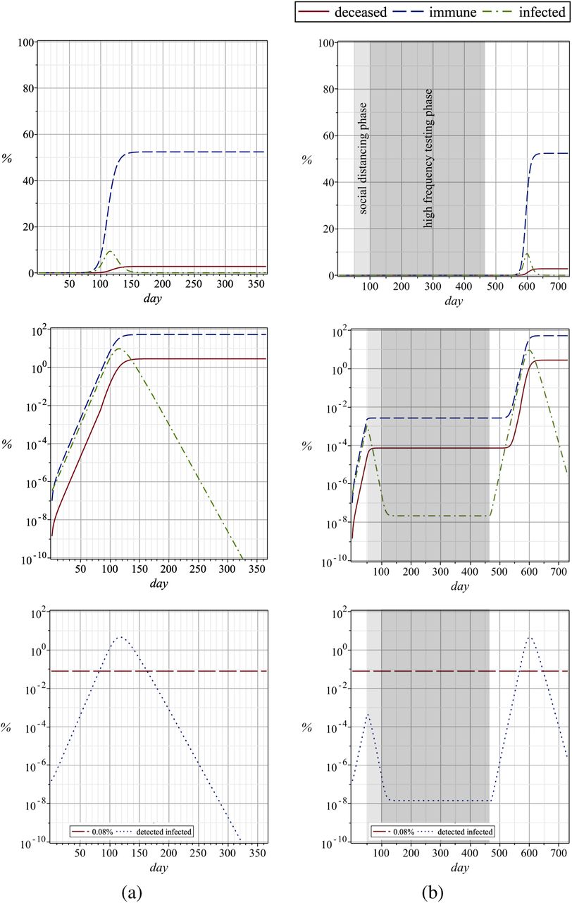
The second mitigation strategy we investigated is mass testing with isolation of detected cases. The same periods as in the cases of Figs. 5a and 5b are considered; once with a 1.7666 times higher detection rate (corresponding to a reproduction factor of one) and once with a 2.8240 times higher detection rate (same reproduction number as with 70% lower infection rate), respectively. The results are shown in Fig. 6 and one can see that they are very similar as those shown in Fig. 5. This demonstrates that mass testing would have a similar effect as social distancing, and provided effective testing methods become available, this approach has the important advantage that the world’s economy would not come to a halt. Like in the case of social distancing, unless one assumes that the virus can be defeated completely and globally, testing would have to be continued until an effective vaccine becomes widely available. Again, information regarding intensive care unit capacity is provided in the bottom logarithmic plots of Fig. 6.

High frequency testing strategy studies. (a): base case (b): 1.7666 times higher detection rate (corresponding to a reproduction factor of one) in the period from 50 to 200 days. (c): 2.8240 times higher detection rate (same reproduction number as with 70% lower infection rate; see Fig. 5) in the period from 50 to 100 days. Dashed lines represent the immune (ns,init − ns(t)), dash-dotted lines the infected (ni|u + ni|d) and solid lines the deceased (nk) population; on the top with linear and in the middle with logarithmic scaling. In the bottom logarithmic plots the detected infected population (dotted lines) is shown together with the intensive care unit capacity (horizontal long dashed lines). The values are in % of the susceptible population size and are plotted over number of days. The gray shading marks the “more frequent testing” phases.
As a final mitigation strategy, we investigated a combination of social distancing and mass testing, i.e., from day 50 to 100 a 70% lower infection rate due to social distancing is considered, followed by a one year period with 1.7666 times higher detection rate. The corresponding plots are shown in Fig. 7. One can see that extreme social distancing brings the number of infections down and moderate testing keeps the values constant. Again, after the testing phase ends there is a delayed outbreak leading to the same end result as in the base case. In the bottom logarithmic plots of Fig. 7 the detected infected population (dotted lines) is shown together with the intensive care unit capacity (horizontal long dashed lines).

Combined strategy study. (a): base case (b): social distancing phase with 70% lower infection rate (50 to 100 days) followed by one year of high frequency testing with a 1.7666 times higher detection rate. Dashed lines represent the immune (ns,init− ns(t)), dash-dotted lines the infected (ni|u + ni|d) and solid lines the deceased (nk) population; on the top with linear and in the middle with logarithmic scaling. In the bottom logarithmic plots the detected infected population (dotted lines) is shown together with the intensive care unit capacity (horizontal long dashed lines). The values are in % of the initial susceptible population size and are plotted over number of days. The light and dark gray shadings marks the “social distancing” and “more frequent testing” phases, respectively.
5. How the Number of Tests Translates to Detection Rate
Finally, we have analyzed how many tests are needed to mitigate the Covid-19 pandemic. How can we achieve the 1.7666-fold increased detection rate modeled in Fig. 6c? To answer this central question, we have studied the relationship between the detection rate kd, i.e., the rate of the identification of infected persons by testing (or by onset of severe symptoms), and the testing interval of the susceptible population.
Obviously, the scenario that the whole susceptible population is tested at once would lead to a trivial disease free state. However in the absence of such capacity, individuals would be tested at different schedules. Let us consider a situation where each person is tested once every N days. Therefore we focus on the set of days 𝒟= { 1, …, N}. An individual is infected at some random time x. To characterize x, we assume that the likelihood of getting infected does not vary much during these days. This is exactly the case, if testing is applied at an intensity such that ℛ0 = 1; see Fig. 7c. Hence x becomes uniformly distributed in the interval [1, N]. The incubation time, which is the time xs between infection and the onset of symptoms, is assumed to obey a log-normal distribution [12]. We assume an incubation time of xs = 5.84 ± 2.98 days [8]. Moreover, we suppose that the testing result becomes available 1/2-day after the test is taken, and that the results are free from false negatives and false positives. The problem of testing frequency hence is reduced to finding N satisfying
 where 𝔼[ . ] denotes expectation. Accordingly, we can find the mean detection time Td as

The above equations are nonlinear (due to the non-linearity of the log-normal distribution) and do not admit closed form expressions for N or Td. Yet, using Monte-Carlo sampling, the maps N−1 → kd and N−1 → Td can be plotted as shown in Fig. 8. As indicated in Fig. 8, increasing the detection rate by 1.7666-fold would require testing the entire susceptible population roughly once every 10 days. This testing interval would suffice to end the pandemic, even if no other mitigation strategies were applied. It is of practical relevance that this is equivalent to testing a random fraction of 10% of the whole susceptible population every day.

Average detection time and detection rate versus testing frequency. Note that the testing scenarios A, B and C are equivalent to testing random fractions of 1/7, 1/14 and 1/30, respectively, of the entire susceptible population every day.
Note that this result can also be applied to situations where only a fraction r is participating in the testing campaign. Then the effective mean detection rate is the weighted average of the detection rate without and with testing, that is,

6. Conclusion
While more and more affected populations are moving from containment towards risk mitigation plans for Covid-19, it is important to understand the engaged mechanisms underlying this pandemic-spread. Outcomes of social distancing and mass testing are investigated in this paper. It is found that the latter can significantly reduce the percentage of people getting infected and the death toll. It is important to emphasize here that more testing has to be applied to individuals without symptoms, since those with symptoms contain themselves automatically in most cases. As improved testing capacities are built up, our approach may help to decide when alternative mitigation methods may not only complement, but eventually replace the current social distancing regime. This may help to minimize the socio-economical impacts resulting from severe social isolation policies. While social distancing is currently essential, it is of utmost importance that the testing capabilities are upgraded such that they cover large portions of affected populations in the near future.
From our analysis we conclude that testing every individual without symptoms roughly every 10 days would reduce the reproduction number of Covid-19 to one and thereby stabilize the pandemic, which is very promising. After a while, fewer and fewer infected people (who spread the virus) will be detected. In this way, continued large scale testing can verify the success of the mitigation strategy. Mass testing should be continued beyond this point, though at a reduced frequency. This would allow to detect if the fraction of infected person tends to increase. If this were the case, testing frequencies should again be ramped up. In any case, unless the virus can be defeated completely and globally by reducing the number of infected individuals to zero, there is a risk of Corvid-19 re-emergence after such mitigation measures are abandoned.
It remains to be emphasized that no claims are made regarding the quantitative accuracy of the presented model predictions, but it can be expected that the qualitative dynamic behavior and the tendencies are captured well. For further improvements of the predictions a more reliable data base for parameter tuning would be necessary. The model itself can be refined by accounting for different age groups and latency, which would involve additional parameters. In the future it would be of utmost interest to further investigate combined strategies with e.g. social distancing for old and endangered persons and high rate testing for the remaining population, including the work force.
Data Availability
All data used for preparation of this manuscript is publicly available.
Acknowledgement
The authors are very thankful to Dario Ackermann, who created the website 3 with the simulation tool based on the model presented in this paper, and the authors would like to thank Emma Slack for helpful comments on the manuscript.


