Abstract
A mathematical model for two strains of Malaria and Cholera with optimal control is studied and analyzed to assess the impact of treatment controls in reducing the burden of the diseases in a population, in the presence of malaria drug resistance. The model is shown to exhibit the dynamical property of backward bifurcation when the associated reproduction number is less than unity. The global asymptotic stability of the disease-free equilibrium of the model is proven not to exist. The necessary conditions for the existence of optimal control and the optimality system for the model is established using the Pontryagin’s Maximum Principle. Numerical simulations of the optimal control model reveal that malaria drug resistance can greatly influence the co-infection cases averted, even in the presence of treatment controls for co-infected individuals.
1 Introduction
Malaria is one of the febrile illnesses and the most common deadly disease in the world caused by one or more species of plasmodium. These are Plasmodium falciparum, Plasmodium vivax, Plasmodium ovale, Plasmodium malariae, and Plasmodium knowlesi. Approximately half of the world population is at risk of malaria. Most of malaria cases and deaths occur in sub-Saharan Africa [1]. According to the World Malaria Report 2018, there were about 228 million cases of malaria and an estimated 405 000 deaths in 2018 [2]. More than 50% of all cases were reported in six countries in Africa, with Nigeria recording 25% of the total global cases. Other African countries include Democratic Republic of Congo (12%); Uganda (5%); Cote d’Ivoire, Mozambique and Niger (4% each) [2].
Cholera is an acute, diarrheal disease caused by infection of the intestine with the toxigenic bacterium Vibrio cholerae serogroup O1 or O139. About 2.9 million persons are estimated to be infected worldwide, with roughly 95,000 deaths annually [3]. Mostly, the infection is mild or without symptoms, although can sometimes be severe. “Approximately 10% of those infected with the cholera will develop severe disease characterized by profuse watery diarrhea, vomiting, and leg cramps. In these people, rapid loss of body fluids leads to dehydration and shock. Without treatment, death can occur within hours” [3].
Mathematical models have been used extensively in studying the behaviour of infectious diseases [4, 5, 6, 7, 8, 9, 10, 11]. A lot of models have been developed for the dynamics of the co-infections of two diseases [12, 13, 14, 15, 16, 17, 18]. In this study, we shall be investigating the impact of malaria drug resistance on the co-infection malaria and cholera, using a mathematical model. Furthermore, optimal control analysis shall be carried out on the model to assess the impact of some control strategies.
2 Model formulation
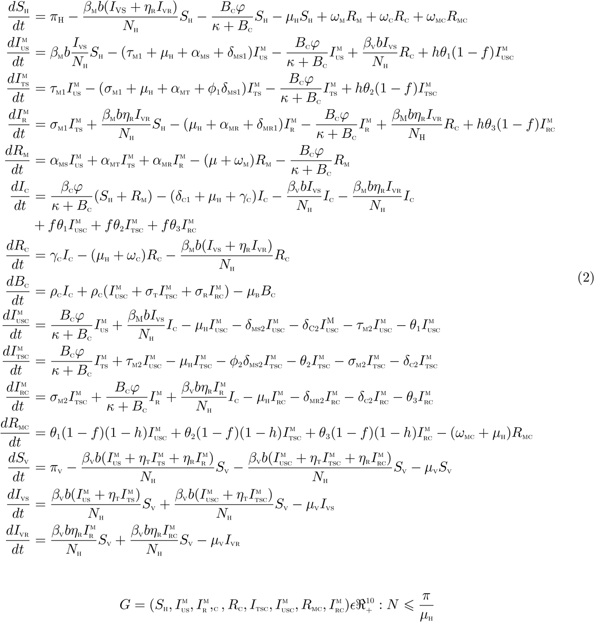
The total human population at time t, denoted by NH(t), is divided into eleven mutually exclusive classes, namely: susceptible humans (SH(t)), untreated individuals with the sensitive malaria strain  , individuals treated of sensitive malaria strain
  , infectious individuals with resistant malaria strain
  , individual that recovered from malaria infection RM(t)), indivdiduals with cholera infection (IC(t)), individuals who have recovered from cholera (RC(t)), individuals untreated of sensitive malaria and infected with cholera,
  , infectious individual treated of sensitive malaria but with cholera infection
  , individual with drug resistant malaria and cholera
  , individuals who have recovered from both malaria and cholera (RMC(t)). Thus

The total vector population NV is divided int three mutually exclusive classes: susceptible vectors, SV, vectors infected with the sensitive malaria strain, IVS, vectors infected with the resistant malaria strain IVR. Thus, NV = SV + IVS + IVR. Also, the bacteria population is given by (BC). Hence, the two strain malaria-cholera co-infection model is given by the following system of deterministic differential equations (the flow diagram of the model is shown in Figure 1 and the associated variables and parameters of the model are presented in Tables1 and 2, respectively):
Schematic diagram of the model (2), with  ,
,  ,
,  ,
,  ,
, 
Description of variables in the model equation
Description of parameters in the model (2).
3 Mathematical analysis of the co-infection model
In this section, we qualitatively analyze the model (2) to better understand the dynamics of the co-infection of drug-resistant Malaria and cholera in a population.
3.1 Basic properties of the Malaria-Cholera co-infection model
3.2 Positivity and boundedness of solutions
For the model (2) to be epidemiologically meaningful, it is important to prove that all its state variables are non-negative for all time (t). In other words, solutions of the model system (2) with positive initial data will remain positive for all time t > 0.
Theorem 3.1
Let the initial data SH > 0,  ,
,  ,
,  , RM > 0, IC > 0, RC > 0, BC > 0,
  ,
,  ,
,  , RMC > 0, SV > 0, IVS > 0, IVR > 0. Then the solution of the model are positive for all t > 0
Proof
Let
t1 = sup{t > 0: SH > 0,  ,
,  ,
,  , 0, RM > 0, IC > 0;RC > 0;BC > 0;
  ,
,  ,
,  , RMC > 0, SV > 0; IVS > 0; IVR > 0 ∈ [0; t]}. Thus, t1 > 0.
We have, from the first equation of the system (2) that
 which can be re-written as

Hence:
 so that

Similarly, it can be shown that:
 ,
,  ,
,  , RM > 0, IC > 0, RC > 0, BC > 0,
  ,
,  ,
,  , RMC > 0, SV > 0, IVS > 0, IVR > 0.
3.3 Invariant regions
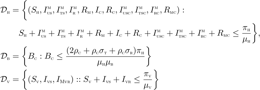
The co-infection model (2) will be analyzed in a biologically feasible region as follows. We first show that the system (4) is dissipative in a proper subset  . The system (2) is split into two parts, namely the human population (NH) (with
  ), the bacteria population, BC and the vector population, (NV) (with NV = SV + IVS + IVR).
The following steps are followed to establish the positive invariance of  (i.e. solutions in
  remain in
  for all time t > 0).
Adding human, bacteria and vector components of the differential system (2), respectively, gives

From (3), we have that
 where δH = min{δMS1, ϕ1δMS1, δMR1, δC1, δMS2, δC2, ϕ2δMS2, δMR2}
Using the Comparison theorem [19], we have that, and
and  if
if  and
and  respectively. Thus, the region
  is positively invariant. Hence, it is sufficient to consider the dynamics of the flow generated by the system (2) in
  . In this region, the model can be considered as being epidemiologically and mathematically well-posed [20]. Thus, every solution of the model (2) with initial conditions in
  remains in
  for all time t > 0. Therefore, the ω-limit sets of the system (2) are contained in
  . Thus result is summarized thus.
Lemma 3.1
The region  is positively-invariant for the model (2) with initial conditions in
  .
.
3.4 Basic reproduction number of the co-infection model (2)
The Malaria-Cholera co-infection model (2) has a DFE, obtained by setting the right-hand sides of the equations in the model (2) to zero, given by

The matrices F and V, for the new infection terms and the remaining transfer terms, evaluated at the disease free equilibrium (DFE) are, respectively, given by
 where
where
H1 = τM1 + µH + αMS + δMS1, H2 = σM1 + µH + αMT + ϕ1δMS1, H3 = µH + αMR + δMR1, H4 = δC1 + µH + γC H5 = µH + δMS2 + δC2 + τM2 + θ1, H6 = ϕ1δMS2 + µH + θ2σM2 + δC2, H7 = δMR2 + µH + δC2 + θ3
The basic reproduction number of the Malaria-Cholera co-infection model (2), using the approach illustrated in van den Driessche and Watmough [21], is given by  where
where  and
and  are, respectively, the Malaria and Cholera associated reproduction numbers, given by
 and
and

3.5 Local asymptotic stability of disease-free equilibrium (DFE) of the co-infection model (2)
Lemma 3.2
The DFE, ξ0, of the Malaria-Cholera co-infection model (2) is locally asymptotically stable if  , and unstable if
  .
.
Proof
The local stability of the co-infection model is analysed by the Jacobian matrix of the system (2) at ξ0, given by:
 with,
with,
H1 = τM1 + µH + αMS + δMS1, H2 = σM1 + µH + αMT + ϕ1δMS1, H3 = µH + αMR + δMR1, H4 = δC1 + µH + γC H5 = µH + δMS2 + δC2 + τM2 + θ1, H6 = ϕ1δMS2 + µH + θ2σM2 + δC2, H7 = δMR2 + µH + δC2 + θ3
G1 = hθ1(1 − f), G2 = hθ2(1 − f),G3 = hθ3(1 − f), G4 = θ1(1 − f)(1 − h), G5 = θ2(1 − f)(1 − h) G6 = θ3(1 − f)(1 − h), D1 = µH + ωM, D2 = µH + ωC, D3 = µH + ωMC, 
The eigenvalues are λ1 = −D1, λ1 = −D2, λ3 = −D3, λ4 = −H5, λ5 = −H6, λ6 = −H7, λ7 = −µH, λ8 = −µV and the solutions of the characteristic polynomials:

 and
and

Applying the Routh-Hurwitz criterion, the quadratic equations (5), (6) and (7) will have roots with negative real parts if and only if  . As a result, the disease-free equilibrium, ξ0 is locally asymptotically stable if
  .
.
3.6 Global asymptotic stability(GAS) of the disease-free equilibrium(DFE) ξ0 of the co-infection model (2)
The approach illustrated in [22] is used to investigate the global asymptotic stability of the disease free equilibrium of the co-infection model. In this section, we list two conditions that if met, also guarantee the global asymptotic stability of the disease-free state. First, system (2) must be written in the form:
 where X ∈ Rm denotes (its components) the number of uninfected individuals and I ∈ Rn denotes (its components) the number of infected individuals including latent, infectious, etc. U0 = (X*, 0) denotes the disease-free equilibrium of this system. The conditions (H1) and (H2) below must be met to guarantee local asymptotic stability:
(H1): For
 , X*is globally asymptotically stable (GAS),
(H2): G(X, I) = AI − Ĝ(X, I)X, G(X, I) ≥ 0 for (X, I) ∈ Ω,
where A = D1G(X*, 0) is an M-matrix (the off-diagonal elements of A are nonnegative) and Ω is the region where the model makes biological sense. If System (2) satisfies the above two conditions then the following theorem holds:
Theorem 3.2
The fixed point U0 = (X*, 0) is a globally asymptotic stable (GAS) equilibrium of (2) provided that R0 < 1 (LAS) and that assumptions (H1) and (H2) are satisfied
 where X denotes the number of non-infectious individuals and I denotes the number of infected individuals.
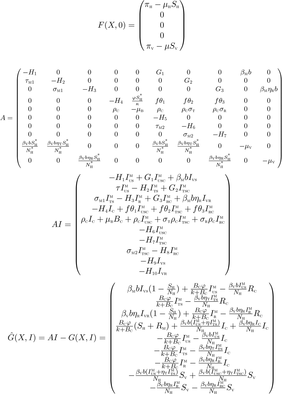
It is clear from the above, that, Ĝ(X, I) ≱ 0. Hence the DFE may not be globally asymptotically stable, suggesting the possibility of a backward bifurcation.
3.7 Backward bifurcation analysis of the full co-infection model (2)
In this section, we shall seek to determine the type of bifurcation the model (2) will exhibit, using the approach illustrated by Castillo-Chavez and Song [23]. We establish the result below
Theorem 3.3
Suppose a backward bifurcation coefficient a > 0, (with a defined below), when 
 then model (2) undergoes the phenomenon of backward bifurcation at
  . If a < 0, then the system (2) exhibits a forward bifurcation at
  .
.
Proof
Suppose
 represents any arbitrary endemic equilibrium of the model. The existence of backward bifurcation will be studied using the Centre Manifold Theory by Castillo-Chavez and Song [23]. To apply this theory, it is appropriate to do the following change of variables.
Let
SH = x1,  ,
,  ,
,  , RM = x5, IC = x6, RC = x7, BC = x8,
  ,
,  ,
,  , RMC = x12, SV = x13, IVS = x14, IVR = x15
Moreover, using the vector notation
 the model (2) can be re-written in the form
 as follows:

 with,
with,
H1 = τM1 + µH + αMS + δMS1, H2 = σM1 + µH + αMT + ϕ1δMS1, H3 = µH + αMR + δMR1, H4 = δC1 + µH + γC H5 = µH + δMS2 + δC2 + τM2 + θ1, H6 = ϕ1δMS2 + µH + θ2σM2 + δC2, H7 = δMR2 + µH + δC2 + θ3
G1 = hθ1(1 − f), G2 = hθ2(1 − f),G3 = hθ3(1 − f), G4 = θ1(1 − f)(1 − h), G5 = θ2(1 − f)(1 − h) G6 = θ3(1 − f)(1 − h), D1 = µH + ωM, D2 = µH + ωC, D3 = µH + ωMC, 
Consider the case when  . Assume, further, that thee product βMηR is chosen as a bifurcation parameter. Solving for βMηR = β* from
  gives
gives

Evaluating the Jacobian of the system (9) at the DFE, J(ξ0), and using the approach in Castillo-Chavez and Song [23], we have that J(ξ0) has a right eigenvector (associated with the non-zero eigenvalue) given by
 where,
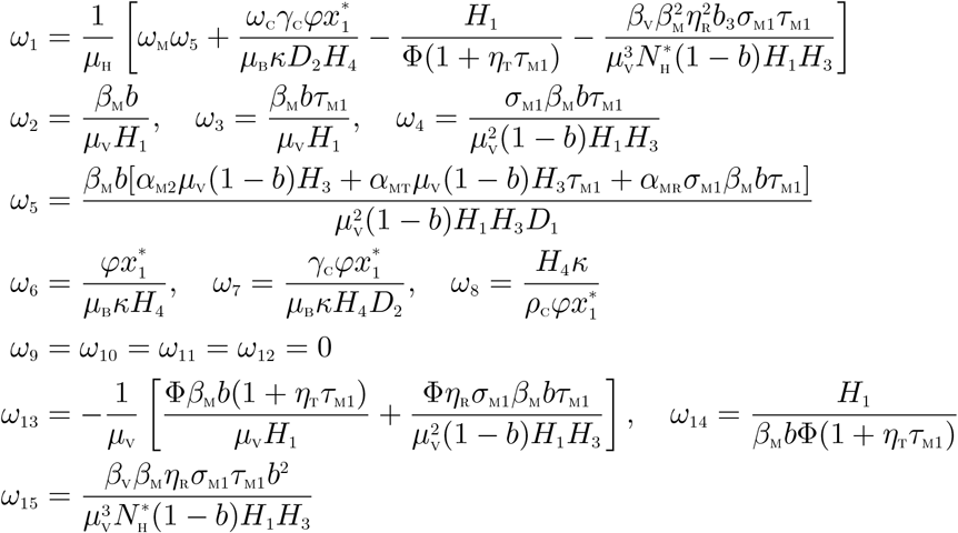
Similarly, the components of the left eigenvector of  , satisfying v.w = 1, are given by:

The non-zero second partial derivatives of the functions fi(i = 1,…, 15) are given by

The associated bifurcation coefficients defined by a and b, given by:
 are computed to be
 and
and

Since the bifurcation coefficient b is positive, it follows from Theorem 4.1 in Castillo-Chavez and Song [23] that the model (2), or the transformed model (9), will undergo the phenomenon of backward bifurcation if the coefficient, a, given by (10) is positive.
4 Analysis of the optimal control model
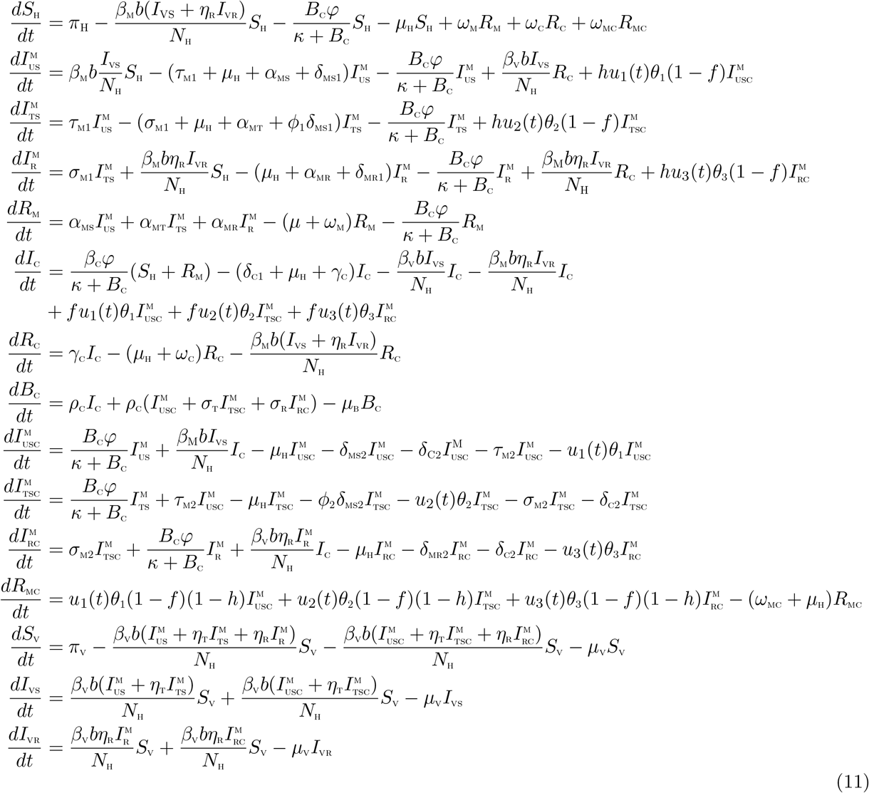
The control functions, u1(t), u2(t), and u3(t) are bounded, Lebesgue integrable functions. The control u1(t) represents treatment efforts for co-infected individuals in  compartment. u2(t) represents treatment efforts for co-infected individuals in
  compartment. The control u3(t) represents treatment efforts for co-infected individuals in
  compartment. The controls u1, u2,u3 satisfies 0 ≤ u1,u2,u3 ≤ 1. The optimal control system examines scenarios where the number of co-infected cases and the cost of implementing the controls u1(t),u2(t), and u3(t) are minimized subject to the state system (11). For this, we consider the objective functional

T is the final time. We seek to find an optimal control,  ,
,  ,
,  , such that
 where
where  such that
  ,
,  ,
,  are measurable with
  ,
,  ,
,  , for t ∈ [0, T] is the control set. The Pontryagin’s Maximum Principle [28] gives the necessary conditions which an optimal control pair must satisfy. This principle transforms (11), (12) and (13) into a problem of minimizing a Hamiltonian,
  , pointwisely with regards to the control functions, u1, u2, u3:

Theorem 4.1
For an optimal control set u1; u2, u3 that minimizes J over U, there are adjoint variables, λ1; λ2,…, λ15 satisfying
 and with transversality conditions

Furthermore,

Proof of Theorem 4.1
Suppose  is an optimal control and SH,
  ,
,  ,
,  , RM, IC, BC,
  ,
,  ,
,  , RUS, SV, IVS, IVR. are the corresponding state solutions. Applying the Pontryagin’s Maximum Principle [28], there exist adjoint variables satisfying:
 with transversality conditions;
 We can determine the behaviour of the control by differentiating the Hamiltonian,
  with respect to the controls(u1, u2, u3, u4) at t. On the interior of the control set, where 0 < uj < 1 for all (j = 1,2, 3, 4), we obtain

Therefore, we have that [29]


5 Numerical simulations
Figure 2 shows the simulation of the total number of individuals untreated of sensitive strain and coinfected with cholera, when there is no drug resistance. it is observed that a total of 1,590 co-infected cases were averted. However as presented in Figure 3 when there is drug resistance, a total of 237 co-infection cases were averted. figure 4 shows the simulations of the total number of individuals treated of sensitive malaria strain and co-infected with cholera. It is observed that a total of 2,527 co-infection cases were prevented, when there is no resistance. However, when there is malaria drug resistance, as depicted figure 5, a total of 116 co-infection cases were averted. Figure 6 depicts the simulations of the total number of individuals co-infected with resistant malaria and cholera. It is seen that in the absence of malaria drug resistance, the treatment control applied prevented a total of 36,350 co-infection cases. However, in the presence of malaria drug resistance, as shown Figure 7 a total of 40,590 co-infection cases were averted when the treatment control is applied. It is imperative to note that in the presence of treatment controls, more co-infection cases were averted when there is drug resistance, than whne there is no drug resustance, for co-infected individuals in compartments  and
and  . However, it is observed that for co-infected individuals in compartment
  , more co-infection cases were averted in the presence of malaria drug resistance than when there is no drug resistance, when treatment controls are applied in both cases. This points to the fact that malaria drug resistance can greatly influence the co-infection cases averted, even in the presence of treatment controls for co-infected individuals.
Figure 8 shows the simulation of the total number of infected individual at different initial conditions. It is observed that the resistant strain drives the sensitive strain to extinction when both reproduction numbers are greater than unity, with  . both strains co-exist with the sentitive strains dominating the resistaant strain when both reproduction number are greater than umity
  . Likewise when both reproduction numbers are greater than unity with
  ,both strain co-exist with th sensitive strain dominating but not driving the resistant strain to extinction.
6 Conclusion
In this work, we have considered and analyzed a mathematical model for two strains of Malaria and Cholera with optimal control. The model assessed the impact of treatment controls in reducing the burden of the two diseases in a population, in the presence of malaria drug resistance. The model was shown to exhibit the dynamical property of backward bifurcation when the associated reproduction number is less than unity. The global asymptotic stability of the disease-free equilibrium of the model was proven not to exist. The necessary conditions for the existence of optimal control and the optimality system for the model is established using the Pontryagin’s Maximum Principle. Numerical simulations of the optimal control model revealed that malaria drug resistance can greatly influence the co-infection cases averted, even in the presence of treatment controls for co-infected individuals
Footnotes
Authors names rearranged properly in Medrxiv


