
Abstract
Solar UV-C photons do not reach Earth’s surface, but are known to be endowed with germicidal properties that are also effective on viruses. The effect of softer UV-B/A photons, which reach the Earth’s surface, on viruses are instead little studied.
Here we show that the evolution and strength of the recent SARS-Cov-2 pandemics, might have been modulated by the intensity of UV-B/A Solar radiation hitting different regions of Earth during the diffusion of the outbreak. Our results suggest that Solar UV-B/A may play an important role in planning new strategies of confinement of the epidemics.
Introduction
It is well known that 200-290 nm ultraviolet photons (hereinafter UV-C radiation) photo-chemically interacts with DNA and RNA and are endowed with germicidal properties that are also effective on viruses [1-8]. Fortunately, Solar UV-C photons of this wavelength are filtered out by the Ozone layer of the upper Atmosphere, at around 35 km [9]. Softer UV photons from the Sun with wavelengths in the range 290-320 nm (UV-B) and 320-400 nm (UV-A), however, do reach the Earth’s surface. The effect of these photons on Single- and Double-Stranded RNA/DNA viruses [9-12] and the possible role they play on the seasonality of epidemics [13], are nevertheless little studied and highly debated in alternative or complementarity to other environmental causes [14-19]. Notably though, the effects of both direct and indirect radiation from the Sun needs to be considered in order to completely explain the effects of UV radiations in life processes (with e.g. the UV virucidal effect enhanced in combination to the concomitant process of water droplets depletion because of Solar heat).
Herein we present a number of concurring circumstantial evidence suggesting that the evolution and strength of the recent Severe Acute Respiratory Syndrome (SARS-Cov-2) pandemics [20, 21], might be have been modulated by the intensity of UV-B and UV-A Solar radiation hitting different regions of Earth during the diffusion of the outbreak between January and July 2020. Our findings, if confirmed by more in depth data analysis and modeling of the epidemics, which includes Solar modulation, could help in designing the social behaviors to be adopted depending on season and environmental conditions.
Results
Coronavirus infections were shown to be influenced by seasonal factors including temperature and humidity [22]. However, these factors have not been observed to modulate the geographical pandemics development of the ongoing SARS-CoV-2 infection [23]. Yet, the available data on SARS-CoV-2 contagions show that the ongoing pandemic has a lower impact during summer time and in countries with a high solar illumination. This suggests that UV-B/A Solar photons may play a role in the evolution of this pandemic.
The optical-ultraviolet solar spectrum peaks at a wavelength of about 500 nm, but extends down to much more energetic photons of about 200 nm. Due to photo-absorption by the upper Ozone layer of the Earth’s atmosphere, however, only photons with wavelengths longer than ∼290 nm (those not sufficiently energetic to efficiently photo-excite an O3 molecule and dissociate it into an O2 + O), reach the Earth’s surface [24]. For a given exposure, the daily fluence (flux integrated over a daytime) on Earth of this UV radiation depends critically on Earth location (latitude) and time of the year and results in the potential of Solar UV-B/A photons to inactivate a virus in air (aerosol) or surfaces.
To evaluate this potential on the onset, diffusion and strength of the recent SARS-CoV-2 pandemics, in our analysis we use the action spectrum (i.e. the ratio of the virucidal dose of UV radiation at a given wavelength to the lethal dose at 254 nm see Methods) compiled in 2005 by Lytle and Sagripanti [12], together with UV-B and –A solar radiation measurement estimates on Earth as a function of Earth’s latitude and day of the year (taken from the Tropospheric Emission Monitoring Internet Service – TEMIS – repository of Solar UV data [25]: http://www.temis.nl; see Methods).
Figure 1 shows two world maps with superimposed a τ0 intensity-gradient image, where τ0 is the lethal-time in minutes needed to deliver the D0(SARS-CoV-2)=4.7 J m-2 UV lethal dose measured by our group at the University of Milan (Bianco et al., 2020, submitted, https://doi.org/10.1101/2020.06.05.20123463; see Methods, also for a discussion on the conservativeness of the assumptions made to estimate the τ0). Data refers to 1 January 2020 (top panel) and 1 July 2020 (bottom panel; details in Figure’s caption). On 1 January subtropical regions (latitude angle α<20 degrees) receive UV doses a factor of ∼20 higher than temperate regions in the north hemisphere (α≈30-50 degrees), while the effect greatly mitigates in May and inverts in July.
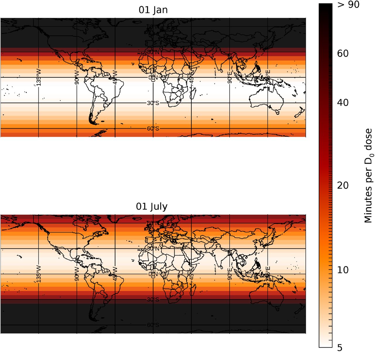
World maps with superimposed a lethal-time intensity-gradient image, as derived from Temis UV-B/A data. Data refers to 1 January 2020 (top panel) and 1 July 2020 (bottom panel). On 1 January subtropical regions (latitude angle α<20 degrees) receive UV doses a factor of ∼20 higher than temperate regions in the north hemisphere (α≈30-50 degrees), while the effect greatly mitigates in May and inverts in July.
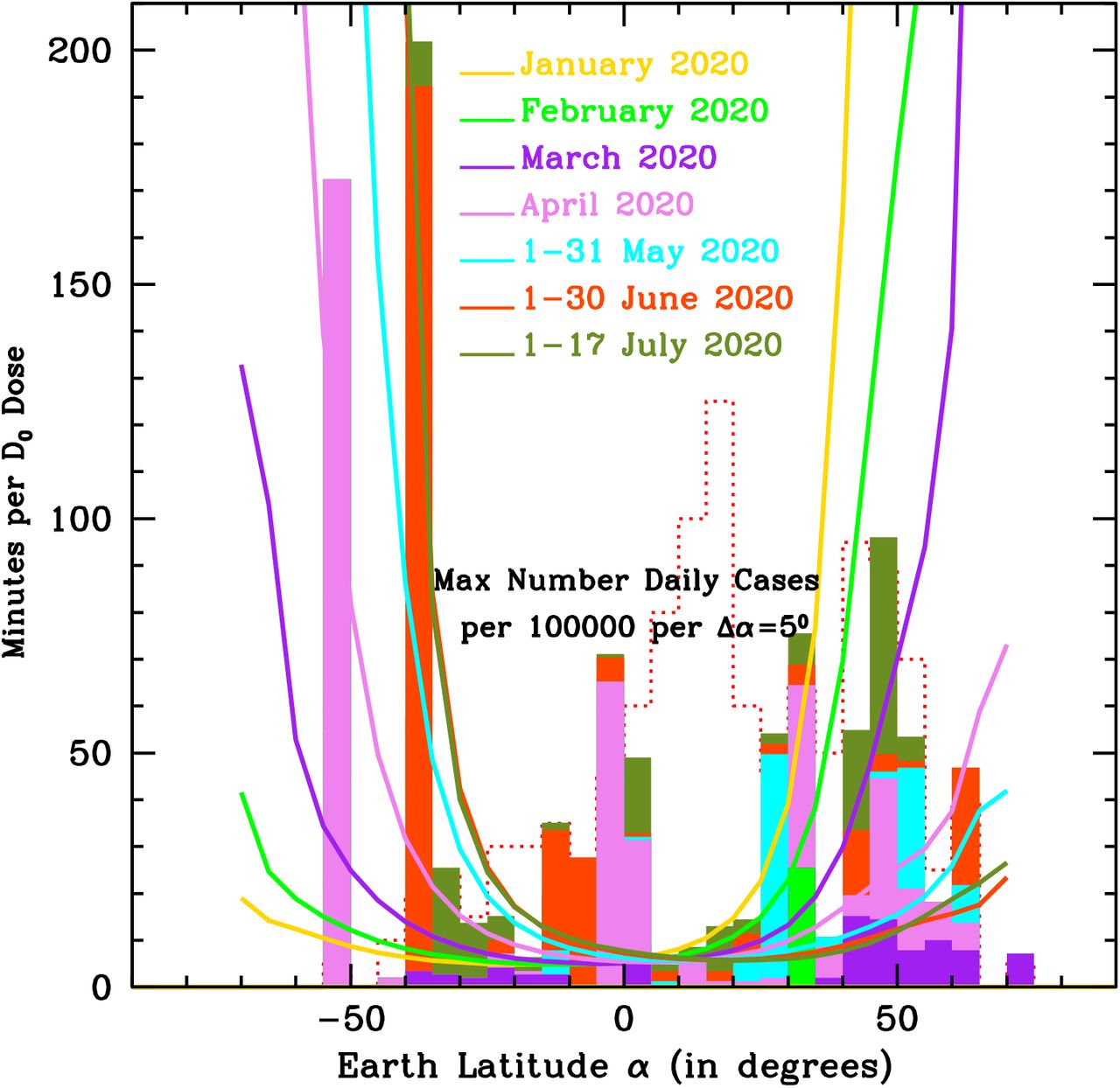
TEMIS data are also used in Figure 2, where the seven curves show the lethal-time τ0, as a function of Earth’s latitude, for the first six months and seventeen days of 2020, as labeled in Figure (see Methods for further discussion). These curves clearly show that during the first three months of the considered period (January1st – July17th), UV-B/A solar photons on Earth’s surface at latitudes −60 < α < −40 degrees are sufficient to inactivate 63% of ss-RNA viruses within 8-to-50 minutes, depending on the exact latitude and time of the year. Between 0.5 and tens of hours are needed instead to obtain the same effect in the same period of the year, at latitudes comprised between α = 40–60 degrees north. The situation is almost reversed in April-July, when > 0.5 hours are needed at −60 < α < −40 degrees whereas 8-40 minutes are sufficient at α = 40–60 degrees north.

The seven curves show the UV-B/A lethal-time τ0, as a function of Earth’s latitude, for the first 6 months and seventeen days of 2020, as labeled. The color-filled histograms shows the maximum number of detected daily SARS-CoV-2 cases per one hundred thousand inhabitants and per Earth’s latitude bins of Δα=50, as of 17 July 2020, in the 229 Countries for which continuous coverage from 22 January 2020 through 17 July 2020 is available. Histogram bins are color-coded according to the month of the year when the maximum was reached in each Country: from February (light green), March (purple) April (violet), May (cyan), June (orange-red) and July (olive-green). Finally, The red, dotted, empty histogram shows the distribution of sampled countries per Δα=50 bins, multiplied by a factor of 5, for easier visualization.
To investigate the effect of this radiation on the diffusion and strength of the SARS-CoV-2 pandemics, we collected COVID-19 data from the GitHub repository provided by the Coronavirus Resource Center of the John Hopkins University (https://github.com/CSSEGISandData/COVID-19). Histograms in Figure 2 show the maximum number of daily detected SARS-CoV-2 cases per hundred thousand inhabitants and per Earth’s latitude bins of Δα=50, as recorded up to July 17th (see Figure’s caption for details). Histograms are color-coded according to the month in which the peak of the epidemic is recorded and in each colored bin, the maximum number of daily recorded cases per hundred thousand is relative to the bottom of the bin (zero-point): for example, the olive-green bin at α=45–50 degrees, starts at a number of daily cases at peak of ≈50 and extends up to ≈95, meaning that the countries at those latitudes which saw the peak of their epidemics in July, reached a maximum cumulated number of daily cases per hundred thousand people of ≈45.
Strikingly, only areas in the north hemisphere show significant peaks of the curves of growth of contagions over the period 22 January – 30 April (light-green, purple and violet histograms). Exceptions are recorded in April (violet histograms in Fig. 2) in the Falkland Islands (α ≈ −53 degrees), where, however, a maximum of only 6 daily cases has been recorded, over a population of only ≈3500 (which makes the number of cases per hundred thousand inhabitant appear outstanding in Fig. 2), and in three high-humidity equatorial countries: Ecuador, a highly populated country with a large number of 11,500 daily cases at peak recorded in April, the rainiest month of the year, Maldives, with only 190 cases recorded at peak over a population of only half million, and Singapore, with a 1426 daily cases at peak, over a population of about 6 million. The situation is almost reversed in May–July, when south hemisphere bins of the histograms of Fig. 2 start to significantly populate. Fig.2 shows also that incidence data on SARS-CoV-2 infection at tropical latitudes, where 99 of the sampled countries are present, was minimal throughout the entire January – July period, with the exceptions of the three countries with peaks in April mentioned above, one country, Peru (where most of the cases have been recorded in densely populated area of the capital, Lima, at a latitude of −12 degrees), with peak in June, and four countries (Columbia, Cameroon, Guinea and French Guiana, with population ranging from only 0.3 million – French Guiana – to 50 million - Columbia) with relatively mild peaks in July. It is important to underline that some of these tropical areas are highly populated and have high average cloud-coverage/day fraction from January through May (central and tropical south America, central Africa and south-east Asia), while the monsoon season starts in May in South India and extends rapidly to the north from May through September.
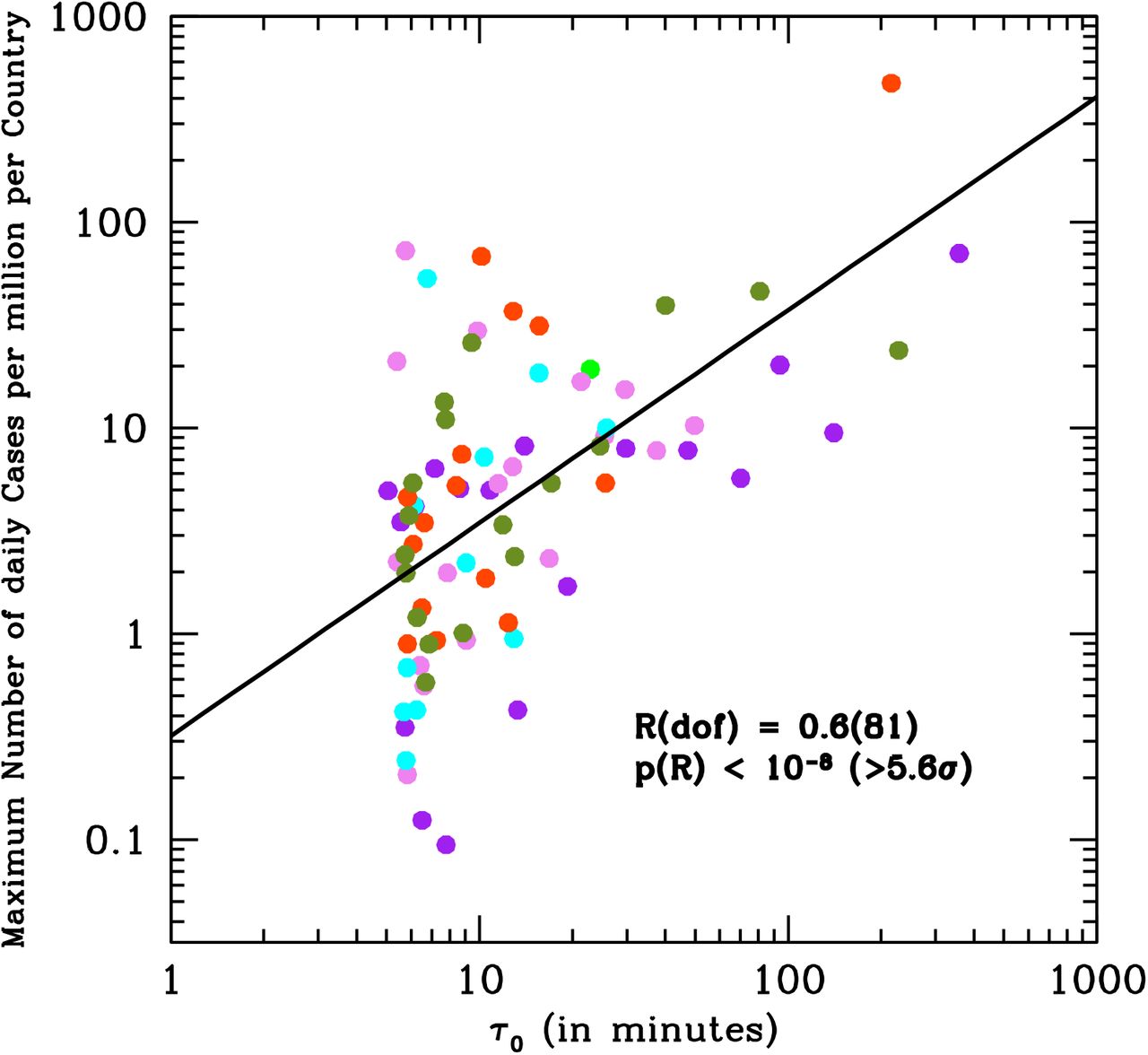
Results are summarized quantitatively in Figure 3, where the maximum number of SARS-CoV-2 cases-per-million and per number of countries per Earth’s latitude bin is shown to correlate with the lethal-time τ0 (see Methods). As expected, given the exponential growth of epidemics and the typical power-law shape of action spectra, this correlation is linear in the adopted log-log space.

Maximum number of daily SARS-CoV-2 case-per-million per Δα=5 degrees bin of Earth’s latitude and per number of Countries per latitude’s bin, as of July 17th in the 229 sampled Countries, versus the lethal-time τ0 as derived from the curves of Fig. 2. Colors indicate the month in which the maximum number of daily cases has been reached: February (light green), March (purple), April (violet), May (cyan), June (orange-red) and July (olive-green).
We did not attempt to correct the data for social-distancing measures (generally adopted more severely by northern Countries, compared to tropical or south Countries) or for tropical daily cloud-coverage (where present during the first six months of the year), which both certainly contribute significantly to the scatter visible in the data. Nonetheless, the correlation in Fig. 3 is statistically highly significant and extends over three orders of magnitudes in τ0 and almost five orders of magnitude in number of SARS-CoV-2 cases. A simple linear-regression Pearson-test of these data-points, yields a null-probability of p<10−8, corresponding to a Gaussian equivalent significance of >5.6σ. The correlation is also present when the number of SARS-Cov-2 cases-per-million is not normalized by the number of countries in the latitude bin, but the statistical significance reduces to 4σ.
The histograms in Fig. 2 are only indicative of the total number density of cases per country, but say little about the growth of the outbreak in each country from their onsets. Figure 4 allows us, instead, to evaluate the momentum of the SARS-Cov-2 epidemics (speed of diffusion times number density of new daily case) in each of the 229 countries sampled (see details in Figure’s caption). Interestingly, onset of the epidemics earlier than 10 March 2020 was only seen in Northern countries, when at these latitudes the minimum exposure needed by UV-B/A photons to inactivate 63% of the virus is longer than 35 minutes (black dotted curve).
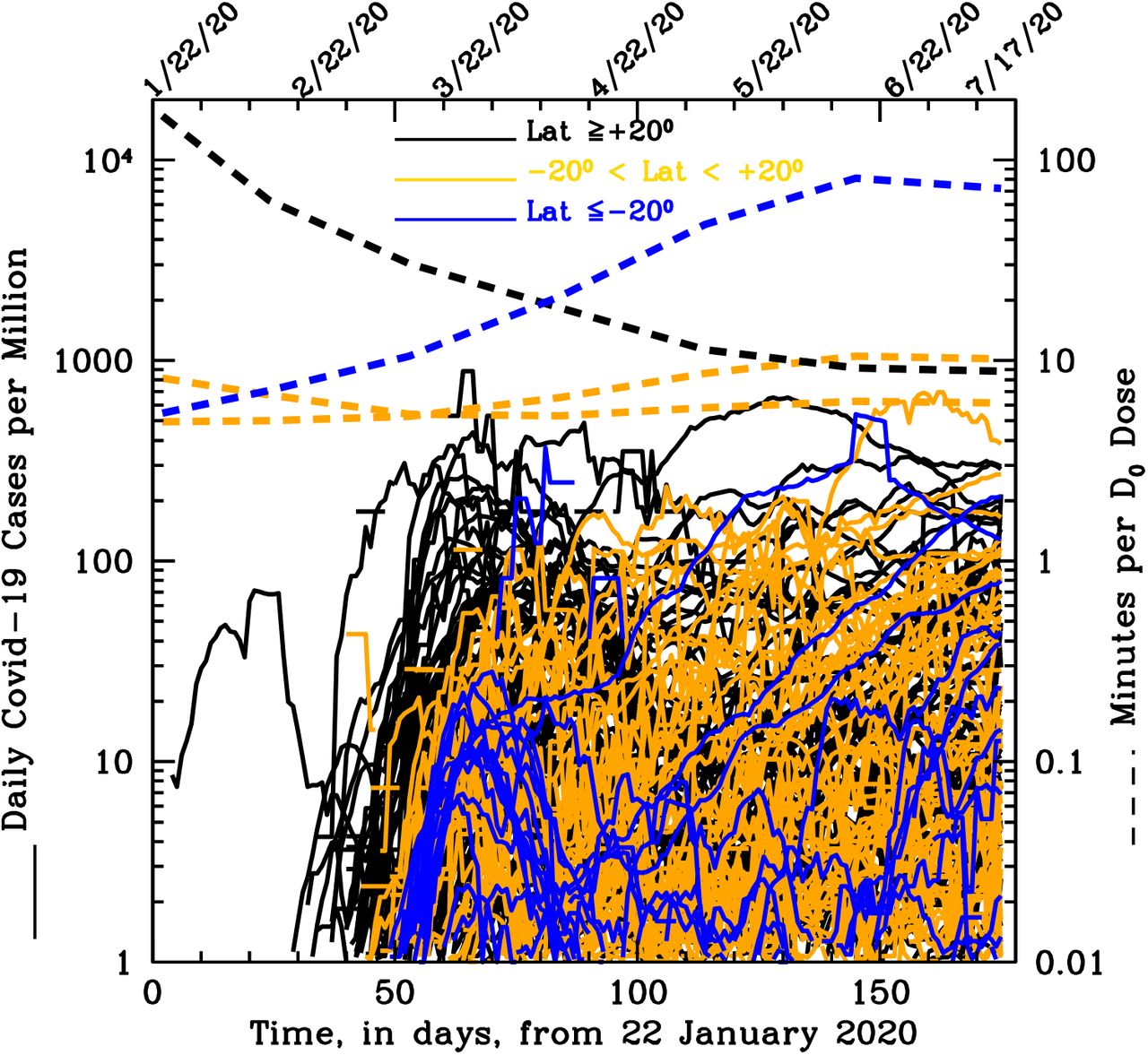
Compilation of the curves of growth of the daily SARS-CoV-2 new cases per million inhabitants in each of the 229 countries sampled. The product between the speed of diffusion and the number of cases cumulated during diffusion is indicative of the momentum of the epidemics in each country. Curves are color-coded according to three broad latitude regions, the North (α>20 degrees, black curves), the South (α<-20 degrees; blue curves) and the Tropical strip (−20 < α < 20 degrees; orange curves). The four additional dashed curves indicate the virus lethal times (in minute: right axis) at α=+40 degrees (black), α=-10 and +10 degrees (orange) and α=-35 degrees (where most of the South countries are located; blue).
Moreover, in Northern countries (black curves) the outbreaks proceeded generally at high rates for tens of days, reached peaks typically higher than a few tens and up to a few hundreds new cases per million people per day (i.e. high momentum, despite the severe measures of social distancing adopted by the majority of these countries) between end of March and mid April, and then started decreasing typically when the minimum UV-B/A virus-inactivation exposure is less than 10–15 minutes.
Discussion
As expected by our model, in South- and Tropical-countries the onset of the outbreak was homogeneously distributed from the end of March through early May (when typical UV-B/A virus-inactivation exposures are between 6-and-30 minutes: yellow and blue dotted curves), and after an initial fast growth the epidemics quickly slowed down, being limited to a few to tens new cases per million people per day (low momentum), to then typically restart in late May through July, when UV-B/A virus-inactivation exposures are between 8-and-80 minutes.
There are a few interesting exception, both in the South and Tropical groups of countries. In the Tropical group, Brazil (where no restriction measures have been adopted till recently), contagions have developed at a high rate from mid March through end of May to then proceed constantly at a slower rate and reach about two hundred new cases per million per day in mid July. The majority of these cases have been recorded in the northern areas of the country, where humidity and cloud-coverage are higher. Peru follows a similar path, but the onset of the epidemics is in April.
In the South group, Chile, Argentina and South Africa after a long initial contained phase of the epidemics that saw no more than a few new cases per million per day (low momentum), SARS-CoV-2 contagions started spreading again towards the end of April (when needed UV-B/A lethal exposures are >30 minutes), and reached values of about 500, 200 and 80 new cases per million per day, respectively between late June and July (increasing momentum).
The segregation by Earth’s latitude of the curves of growth of Figure 4 can be well reproduced qualitatively by simulating the effect of the Sun with Monte-Carlo runs of simple diffusive model solutions, as detailed in Methods and shown in Supplementary Figures S1 and S2.
Taken together, the curves of growth of Figure 4, suggest that the epidemics efficiently develops in areas where typical UV-B/A virus-inactivation exposures are longer than about 30 minutes (but see Methods for the conservativeness of our assumptions on τ0).
This value should be compared to the stability of SARS-CoV-2 on aerosol and surfaces. A recent study shows that SARS-CoV-2 can survive in aerosols for longer than three hours and is even more stable on metallic and polymeric surfaces, where it can stay for up to several tens of hours and is quickly inactivated by solar light [27]. These results, combined with another recent research showing that the lifetime of speech droplets with relatively large size (> few micrometers) can be tens of minutes [28], suggest that SARS-CoV-2 may spread through aerosols (either directly, through inhalation, and/or indirectly, through evaporation of contaminated surfaces).
Our results suggest that Solar UV-A/B might have had a role in modulating the strength and diffusion of the SARS-CoV-2 epidemics, explaining the geographical and seasonal differences that characterize this disease. They also imply, if confirmed, that the UV flux received by our Sun in open areas may represent an important disinfection factor (e.g. [27]), able to significantly reduce the diffusion of the pandemics. This could help in designing new strategies of confinement of the epidemics that may provide better protection with less social costs (see e.g. [20]).
Methods
UV-C Lethal Dose for SARS-CoV-2
In 2005, Lytle and Sagripanti [12] reviewed several experimental studies of inactivation of viruses (including viruses with single- and double-stranded DNA/RNA and ee-stranded genoma) by UV light exposure and reported the mean lethal dose at 254 nm (the UV wavelength at which the maximum inactivation of virus takes place) in terms of fluence (J m-2) needed to inactivate 63% of the virus (D0 hereinafter).
They concluded that the product between the mean lethal dose at 254 nm D0 and the size of the genoma (Size-normalized Sensitivity - SnS) is approximately constant. This means that larger doses of UV radiation are needed to produce the same fraction of inactive viruses with smaller sizes. For the Berne coronavirus, which has genome size of 28 kb, Lytle and Sagripanti [12] report the lethal dose D0=3.1 J m-2 at 254-nm measured by M. Weiss and M.C. Horzinek [29]. Consistently, for the SARS-CoV-2, with a slightly larger genoma-size of 29.8-29.9 kb [30], our experiment at the University of Milan measured a lethal dose D0=4.7 J m-2 at 254-nm (Bianco et al., 2020, submitted, https://doi.org/10.1101/2020.06.05.20123463). This is the D0 value we assume in our work.
Solar Radiation and Microorganisms
The mechanisms through which UV radiation from the Sun acts on viruses and, in general, microorganisms are both endogenous and exogenous and depend on the exact wavelength of the photons. For viruses, the direct endogenous mechanism is the most important, and consists in direct absorption of the UV photon by the chromophore embedded in the virus, as the nucleic acid or protein [31]. This process is known to decrease in efficiency going from UV-C to UV-B and is not active in the UV-A, where only the exogenous mechanism is effective [32].
UV strongly interacts with gaseous and aerosol pollutants in the air affecting the amount of UV radiation reaching the Earth surface. Nitrogen and Sulphur oxides together with Ozone strongly absorb UV light with efficiency increasing from UV-A to UV-B [33,34]. In addition, scattering of light by particles and aerosols is proportional to their concentration and highly polluted areas show again a UV reduction effect that goes in the same direction of molecular absorption.
Solar UV Data
In our analysis, we use Solar UV data made available by the Tropospheric Emission Monitoring Internet Service (TEMIS) archive.
TEMIS is part of the Data User Programme of the European Space Agency (ESA), a web-based service that stores, since 2002, calibrated atmospheric data from Earth-observation satellite. TEMIS data products include measurements of ozone and other constituents (e.g. NO2, CH4, CO2, etc.), cloud coverage, and estimates of the UV solar flux at the Earth’s surface. The latter are obtained with state-of-the-art models exploiting the above satellite data. It should be noted that a depletion of the Ozone stratospheric layer has been observed during the last few decades due to interaction with Cloro-Fluoro-Carbon (CFC) gas emitted in industrial activities, with consequent increase of the atmosphere transparences to UV light [34].
UV-B/A Action Spectrum
Lytle and Sagripanti [12] estimated SnS in the 280-320nm wavelength range for a variety of viruses with known genome compositions and sizes by compiling measurements obtained at longer wavelengths and normalizing them to 254 nm. The final product is the UV-B/A action spectrum, defined as the ratio of the lethal dose at a given wavelength to the dose at 254 nm.
TEMIS UV products include integrated UV doses [in kJ/m2] weighted for different action spectra, normalized at 300 nm. In this study we use TEMIS data folded through the unshielded-DNA damage action spectrum and renormalized to 254 nm. This renormalization brings the two action spectra TEMIS DNA and Lytle and Sagripanti single- and double-stranded RNA/DNA [12] to match in the common 250-320 nm wavelength range, and yields to the virucidal UV-B/A flux Fvir, in J m-2 day-1 used in our analysis.
Lethal Exposure as a function of Earth’s latitude and Time of the year
To obtain the curves of exposure needed to irradiate the lethal dose as a function of Earth’s latitude, we considered the whole TEMIS data set (259 locations around the world) for year 2019 and 2020 and interpolated on a regular latitude grid of 5 degrees. We conservatively considered only the 20% of the Solar flux Fvir released in the one hour interval centred around local noon and computed the virucidal UV flux per minute when the Sun is close to its daily maximum elevation. The lethal exposure, in minutes, is thus given by:
Our Conservative Assumptions
All the approximations we used to compute τ0 are conservative:
the Fvir vs latitude dependence was obtained by excluding locations with altitude > 400 m, where Fvirvalues are higher because of the thinner atmosphere column.
the adopted fraction of 0.2 Fvir is the minimum value obtained by simulating the UV Index (http://www.temis.nl/uvradiation/product/papers/WR2016-01.pdf) for a given instantaneous zenith angle (as a function of latitude and time of the year) and computing the fractional dose released in a one-hour time interval centered on the local noon: for comparison, the mean observed attenuation factor is 0.34 Fvir. Properly distributing the remaining 80% of the daily solar flux in time as a function of latitude and time of the year, would lower the threshold of the minimum lethal exposure.
TEMIS data on broad global scale are only available for clear sky. For Europe and few locations of central America and the south hemisphere cloud correction is available. The difference between cloud corrected and clear sky data show high frequency fluctuations due to weather superimposed to a low frequency seasonality effect (winter/summer modulation in temperate areas and rain/dray seasons in the tropical areas). Considering cloud-coverage would then amplify (in both directions) the observed latitude effect of Solar virucidal power.
aerosols are the main responsible for local Fvirabsorption and scattering and may vary greatly from location to location on Earth. TEMIS data account for this effect by reducing Fvirvia a flat mean attenuation factor of 0.3. Experiments made on ground showed actual doses up to a factor 2 higher than those reported by TEMIS, implying that the adopted flat 0.3 factor is highly conservative (local aerosol measurements would be incredibly interesting to study infection diffusion in polluted areas but this would require specific data per targeted area and are beyond the scope of this analysis).
SARS-CoV-2 Pandemics Data
We collect SARS-CoV-2 data pandemics from the on-line GitHub repository provided by the Coronavirus Resource Center of the John Hopkins University (CRC-JHU: https://github.com/CSSEGISandData/ COVID-19). CRC-JHU global data are updated daily and cover, currently, the course of epidemics in 229 different world countries (and regions for Australia and Canada), by providing the daily cumulated numbers of Confirmed SARS-CoV-2 cases, Deaths and Healings. We use CRC-JHU data run from 22 January 2020 (recorded start of the epidemics in China) through 17 july 2020.
The color-filled histograms of Figure 2 are produced by grouping CRC-JHU global data of confirmed SARS-CoV-2 daily cases per hundred thousand people at peaks as of 17 July 2020, in Earth’s latitude bins of Δα=5 degrees, independently on the Earth’s longitude of the sampled Countries.
The doted red histogram of Figure 2, shows the number of Countries per bin, multiplied by a factor of 5 for easier visualization.
Black (North Countries), orange (Countries in the Tropical strips) and blue (South Countries) curves in Figure 4, are the curves of growth of the daily new confirmed SARS-CoV-2 cases per million people, from the start of epidemics in each Country through July 17th. These curves are derived by first differentiating the cumulative curve of growths provided by CRC-JHU and then operating a non-weighted 7-day moving average on the data, to smooth non-Poissonian daily fluctuations (systematics).
Modeling the Earth’s latitude Segregation of SARS-CoV-2 Cases with Simulations
The segregation by Earth’s latitude of the SARS-CoV-2 curves of growth of Figure 4 can be well reproduced qualitatively by simulating the effect of the Sun with Monte-Carlo simulations of simple diffusive model solutions.
Supplementary Figure S1 shows two runs of such simulations, with (bottom panel) or without (top panel) the solar effect. Simulations are run for 229 countries with latitudes and populations distributed randomly and uniformly accordingly to the three latitude groups in the observed SARS-CoV-2 pandemics data (109 North Countries: black curves; 99 Tropical Countries: orange curves; 21 South Countries: blue curves). Each curve represent the daily number of infections per million inhabitants for a given Country and is the solution of a simple diffusive SIRD-like (Susceptible, Infected, Recovered, Deaths) model, where epidemics starts at a time TStart, lockdown measures are taken at TLD and reopening starts at TOpen. TStart, TLD and TOpen are randomly and uniformly distributed between the intervals labeled in the two panels of Fig S1, as are the halving and doubling times of the reproductive number Rt, before lockdown and reopening, respectively. Lockdowns and re-openings are both modeled with exponential functions that act as attenuating and amplifying factors, respectively, of the daily probability of contacts between individuals, with halving and doubling times T1/2.LD and T2,open.
The two panels of Supplementary Fig. S1 differ only for the absence (top panel) or presence (bottom panel) of the solar effect. The solar effect is introduced as a daily piston, modeled as Gaussian functions which deliver 20% of the UV-B/A Solar flux observed between 1 January 2020 and 17 July 2020 (TEMIS data of Figure 2-4), with a standard deviation of 5 hours centered on local noon and peak-intensity inversely proportional to the lethal-time τ0 (Supplementary Figure S2).
Segregation (by over an order of magnitude) in Earth’s latitude of the simulated daily SARS-CoV-2 infections, qualitatively similar to that observed in real data (Fig. 4), can only be obtained by switching the Sun on (Fig. S1, bottom panel).
Figures’ Production
Figure 1 is produced via scripts written by us in the IDL scripting language (https://www.harrisgeospatial.com/Software-Technology/IDL).
Figure 2–4 and Fig. S1–S2 in the Supplementary Information, are produced via scripts written by us in the scripting language Supermongo (https://www.astro.princeton.edu/~rhl/sm/sm.html).
Data Availability
For the UV illumination data we used public data provided by the TEMIS network http://www.temis.nl/ SARS-CoV-2 data are taken by the GitHub repository provided by the Coronavirus Resource Center of the John Hopkins University: https://github.com/CSSEGISandData/COVID-19
Authors’ Contribution
F.N. prepared Figures 2-4 and 1S-2S. G.S. prepared Fig. 1 and helped preparing Fig. 2. All authors contributed equally to the discussion of the results and review of the manuscript.
Declarations
I confirm that I understand Scientific Reports is an open access journal that levies an article processing charge per articles accepted for publication. By submitting my article I agree to pay this charge in full if my article is accepted for publication.
No, I declare that the authors have no competing interests as defined by Nature Research, or other interests that might be perceived to influence the results and/or discussion reported in this paper.
The results/data/figures in this manuscript have not been published elsewhere, nor are they under consideration (from you or one of your Contributing Authors) by another publisher.
I have read the Nature Research journal policies on author responsibilities and submit this manuscript in accordance with those policies.
Supplementary Information
Supplementary Figures

Monte-Carlo simulations for 229 countries with latitudes and populations distributed randomly and uniformly accordingly to the three latitude groups in the observed SARS-CoV-2 pandemics data (109 North Countries: black curves; 99 Tropical Countries: orange curves; 21 South Countries: blue curves). Each curve is the solution of a simple diffusive SIRD-like (Susceptible, Infected, Recovered, Deaths) model, where epidemics starts at TStart, lockdown measures are taken at TLD and reopening starts at TOpen.. TStart, TLD and TOpen and randomly and uniformly distributed between the intervals labeled in the two panels, as are the halving and doubling times of the reproductive number Rt, before lockdown and reopening, respectively. The two panels differ only for the absence (top panel) or presence (bottom panel) of the Solar effect (see Methods for further details).
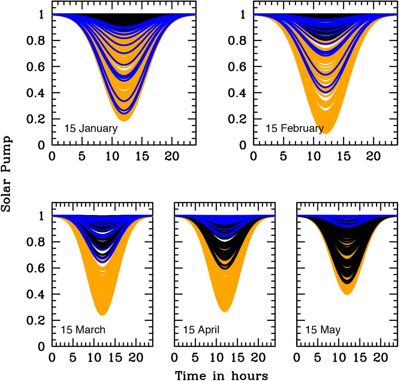
Gaussian functions used to introduce the Solar effect in the simulations of Fig. S1. These Gaussians have all standard-deviation σ=5 hours, peak centered at local noon and intensity inversely proportional to the SARS-CoV-2 lethal-time τ0. They act as a daily disinfecting pump on epidemics by delivering 20% of the UV-B/A Solar flux observed between 1 January 2020 and 17 July 2020 (TEMIS data of Figure 2-4) as lethal photons. Gaussians are plotted for 5 representative days of 2020: the 15th of January, February, March, April and May. The curves are color-coded as in Fig. S1.
Acknowledgments
The work presented in this paper has been carried out in the context of the activities promoted by the Italian Government and in particular, by the Ministries of Health and of University and Research, against the COVID19 pandemic. Authors are grateful to INAF’s President, Prof. N. D’Amico, for the support and for a critical reading of the manuscript. Authors are also grateful to Prof. A. Musarò, Dr. M. Elvis, and Dr. F. Fiore for critically reading the papers and providing useful comments and suggestions.


