EXPECTATION OF LIFE: AN ALTERNATIVE FOR SUMMARISING ALL CAUSES MORTALITY

Length of life was used by William Farr to measure the health of populations over 150 years ago (beginning with the Registrar General's 5th annual report) and to make international comparisons, arguing that the life table was the only correct measure of average length of life, which the early Victorians accepted as a measure of health and vitality1 (although expressed erroneously as the mean age at death). More recently, Gardner and Donnan2 used life expectancy as an alternative to SMRs to illustrate variations in Regional mortality in England and Wales, noting that the range of differences between the Regions was less than differences between men and women, but greater than the change in life expectancy that could result by eliminating cancer mortality. They also thought that expectation of life from birth would “help doctors and laymen alike to grasp the significance of a range of SMRs by using the more familiar terms of years of life lost”. Devis3 compared time trends in the expectation of life from birth and from age 65, in men and women based on current mortality rates—noting that the changes in this “convenient measure of mortality” resulted from the rapid declines in infant and childhood mortality since the Victorian era. Variations in expectation of life at health authority level have also been explored,4 and Craig,5 noting that life expectancy is an average tackled the issue of uncertainty from the viewpoint of the chances of an earlier death than average. Thus a man aged 40 would have an average future life of 35 years but 1% of 40 year old men would die within as little as five years. He also presented variations in median age at death (calculated by life table) by age sex and period. However, his article did not consider the possibility of sampling variation in this estimation. Others6-8 have devised formulas to link the SMR and life expectancy, again motivated by the latter's more ready appreciation by non-specialists.

With a current, demographic life table, life expectancy at birth in a given population is defined as the average length of life of a newborn child if current age specific mortality rates in that population applied in the future. Clearly the true average lifespan would need follow up for over 100 years and such cohort specific life tables would be impractical for routine purposes.

As indicated above, estimation of expectation of life first requires construction of a life table to give the proportion alive at each age x , denoted by L_x. When plotted, the y axis represents the L_x values and the x axis represents age. Often for presentation the values in the life table are multiplied by a convenient large number, for example, 100 000 so that L_xrepresent numbers of persons rather than a proportion—but this is does not affect the algebra.

The expectation of life from birth is given by the area under the life table plot from birth divided by the number originally alive. Likewise expectation of life from any age can be found. Thus in figure 1 the shaded area divided by 0.91 gives the expectation of life from age 60. This is dimensionally correct—the y axis has the dimension of persons, and the x axis has dimension of years so the area under the curve has dimension person years, and when divided by the number alive at a given age the dimension is years. For computational purposes, the area can be estimated by the trapezium rule. While such calculations are tedious by hand, they are easily set up with the aid of a spreadsheet.

• Download figure
• Open in new tab
• Download powerpoint

Figure 1

Principle of estimation of expectation of life from age x . Life expectancy from birth is the area under the life table plot from birth divided by the number originally alive. Likewise expectation of life from any age can be found, for example, the shaded area divided by 0.91 gives the expectation of life from age 60.

Standard textbooks ignore the issue of sampling variation in demographic life tables, although formulas are available for clinical life tables.9 However, these assume all subjects have been followed up until death. When this is not the case, there are a number of solutions10 ranging from taking the estimated proportion of survivors after the longest complete survival time to be zero, (giving a negatively biased estimate), to carrying forward the last observed proportion of survivors. Another suggestion is that the “tail” of the survival curve should be completed by an exponential curve picked to give the same value as the proportion of survivors at the last completed survival time.

This last proposal is superficially related to our approach, but is differently motivated and applied, as will become clear. In fact, none of these suggestions really apply to demographic life tables, where not only the hazard rate is known for the final age band, but it is also known that all people will die within a few years. Another possibility is to model the whole life table 8 but this is unlikely to appeal or be available to the average public health physician.

Obviously sampling variation is not an important issue when national or even regional life tables are constructed. However, to make valid inferences it is clearly important to allow for year to year random variations in the number of events that are observed when comparing mortality at local level, for example, for electoral wards within a health district. Moreover attempts to increase precision by aggregating data over a number of years will degrade the extent to which the data reflect current conditions. Similar issues of sampling variation apply to other summary measures of mortality, such as age standardised rates.

An estimate of the standard error could also be used to indicate how many years worth of data would need to be aggregated to achieve a desired level of precision, and could perhaps be used in statistical analysis. Standard errors for the CMF and the SMR are easily available in standard textbooks, but this is not so for the expectation of life based on demographic life tables.

In addition, the effects of cause specific mortality can be compared using life table methods, which take into account competing risks (unlike comparisons of cumulative rates, which are essentially a form of directly age standardised rate). However, the issues of the shape of the sampling distribution and the effect of closed upper age band would remain.

Results

The formula for the variance of e^o _x was cumbersome, but once set up on a spreadsheet it was not too hard to change the number of age bands for example, and was not much more difficult than setting up a spreadsheet for the SMR and CMF.

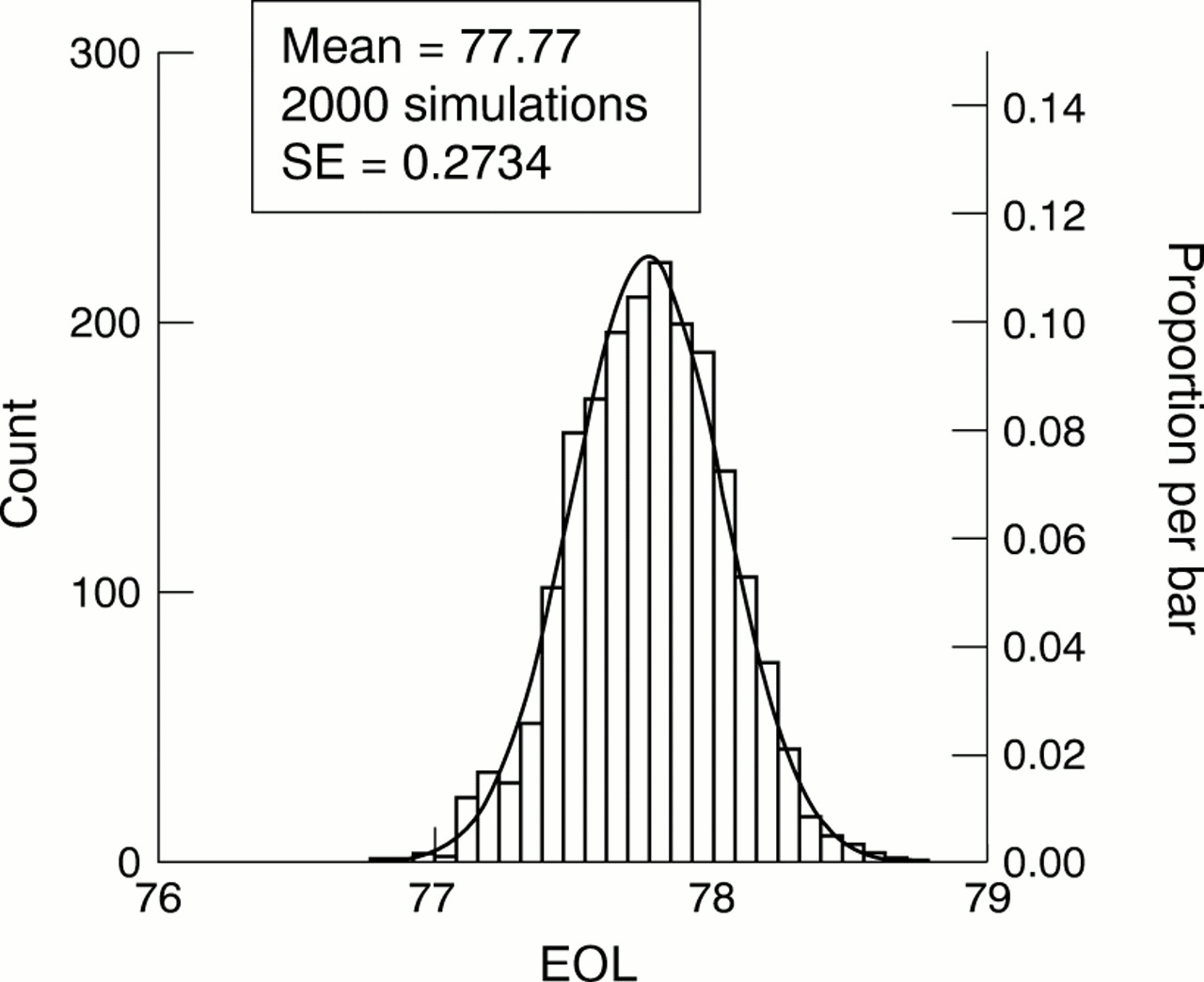
For the test data set our formula gave a standard error of 0.2711, while a simulation (n=2000) gave a value of 0.2734, confirming the accuracy of the formula. The simulation used a normal approximation to the Poisson distribution for values of 100 or more (algorithms in Cooke and Craven11). The sampling distribution of e^o _x was approximately normal (fig2).

• Download figure
• Open in new tab
• Download powerpoint

Figure 2

Simulated sampling distribution of expectation of life from birth if final age band is “open”, with superimposed normal curve.

The expectation of life at 85+ for the life table based on 1990–9212 is 4.8 years for men and 6.1 years for women. The reciprocals of the corresponding mortality rates are 5.2 years and 6.7 years respectively. For the life table based on 1994–9613 the corresponding values are 4.9 years for men and 5.2 years for women with reciprocals of mortality rate of 6.3 years and 6.6 years. The similarity of these values to the reciprocal of the mortality rate in the oldest age band indicated that an exponential assumption for survival in the oldest age band is reasonable.

For fixed upper age limit the sampling distribution was also approximately normal, with standard errors of 0.263 by formula and 0.265 on simulation, slightly smaller than the values found with an open age band—as would be expected.

For small populations some age bands will have zero deaths. The effect will be a spurious decrease in the estimated sampling variation. In addition for such age bands the normal approximation to a Poisson distribution will be invalid, although the effect of these age bands on the overall distribution may be negligible. We explored this with a simulated population of about 28 000 for which there were no deaths in the four age bands from ages 1 to 19. No age band had more than 60 deaths and the Poisson model was simulated without a normal approximation. The standard error based on 2000 simulations was 0.704 (with excellent approximation to normality). The value based on our formula was 0.697.

A possible ad hoc correction for age bands with such “random zeroes” is to impute a small positive value. We tried two alternatives: firstly 0.693 (being the value for the Poisson rate for which the chance of observing 0 events is a half) and secondly a value of 3 (being the upper 95% confidence limit for the frequency of events when none are actually observed). These corrections increased the simulation-based standard error to 0.785 and 0.934 respectively, compared with formula-based values 0.759 and 0.928. Again the approximation to normality was excellent.

ALTERNATIVE MEASURES

1 SMR

This compares the observed deaths in an index population of interest relative to the number to be expected in the index population if age specific deaths rates in the standard (reference) population applied. It is usually expressed as a percentage.

2 Comparative mortality figure

This compares the deaths to be expected in the standard population if age specific deaths rates in the index population applied, relative to the number observed in the standard population.

Both the SMR and the CMF can be shown to be weighted averages of the relative rates in each age band (that is, each age band's mortality rate in the index divided by that in the standard), as shown below where R_i = relative rate in ith age band.

SMR = Σ (n_i M_i) R_i/Σn_i M_i

CMF = Σ (N_i M_i) R_i/ΣN_i M_i

n_i = size of population in index population in ith age band

M_i= mortality rate in standard population in ith age band

N_i = size of population in standard population in ith age band

R_i = relative risk of index compared with standard in ith age band

Advantages of the SMR are:

1

If the relative rates are constant across the age bands and deaths are distributed as a Poisson variate, then the SMR is a minimum variance estimate of the relative rate (in particular its variance is less than that of the CMF).

2

It is not necessary to have details of age bands in which the deaths in the index population occurred.

The key disadvantage of the SMR is that it is inconsistent. Two CMFs will differ only because the age specific relative rates differ, while two SMRs may be unequal because the age structure of the index populations are not the same (which affects the weights used to average the relative rates).

Being forms of relative rate, both indices have a fairly straightforward lay interpretation on the lines of: “in the North West, the risk of death from cervical cancer is 20% greater than the average for England and Wales”

However, both CMF and SMR also require choice of a suitable standard population. For international comparisons “African”, “World” and “European” standard populations have been defined, with correspondingly different age structures.

3 Age standardised rates

It can easily be shown that:

Indirectly age standardised rate = crude rate in standard population × SMR

and

Directly age standardised rate = crude rate in standard population × CMF

Which intuitively is the case because of their interpretation as a relative rate.

In addition to the need for an appropriate standard population, age standardised rates—with one exception (below)—lack an easy lay interpretation unless one is presented with comparison figures. For example there is little information in the statement that “in 1989 the directly standardised incidence rate for colonic cancer in men in Trent Region was 17.6 per 100 000” unless accompanied by the corresponding figure of 18.9 per 100 000 for England and Wales.

An alternative form of direct standardisation, which does not require an arbitrary external standard population and that does have an easy lay interpretation is the cumulative rate.

4 Cumulative rate

This is the sum of the mortality rate in each age band times each age band's width, the sum typically being taken up to and including age 74, but it can be extended to any defined upper age limit.14

For rates less than 10% per year the cumulative rate is a good approximation to the lifetime risk of developing (or dying from) the disease in question—were other causes of death avoided. For higher rates it is easy to convert the cumulative rate to a cumulative risk, using the formula:

cumulative risk = 1−exp(−cumulative rate)

The main disadvantage is that it requires an arbitrary upper age cut off, and that it is most applicable to comparisons of cause specific rates, rather than all causes mortality.

Discussion

In epidemiology the most common parametric procedures are based on an assumption of approximate normality, whether this is in the construction of approximate confidence limits on a cumulative rate for example, or in the comparison of two SMRs. When necessary the approximation can be improved by an appropriate transformation (such as the square root transformation for Poisson variates). Furthermore even the common use of the χ² test, as in the comparison of several proportions, requires an underlying assumption of at least approximate normality because the χ² distribution is itself the sum of independent squared normal deviates.

We obtained the sampling distribution of the expectation of life by simulation and have shown that this is in fact approximately normal, but that the formula for its standard error is too complex for easy “hand calculation” (although it is easy to set up on a spreadsheet). We have also shown that age bands with zero events do reduce the standard error slightly, but without affecting the approximate normality of the expectation of life. Application of corrections to age bands with zero deaths increased the discrepancy between simulated and formula-based standard errors.

The possibility of zero events in some age bands will also occur with other methods for comparing mortality rates. So called computer intensive procedures (of which Monte Carlo simulation is an example) are valuable here when it is not easy to assess analytically the exact effect of such zeroes, or of substituting a small constant. However, such procedures do require investment in extra programming, which may not be justifiable on a routine basis.

An additional problem, common to both standardisation procedures and expectation of life, is that the last age band, typically 85+, is left “open-ended” . As such open-ended age bands can have very different age structures in different populations and can misleadingly imply similarity of risks (table 1) it is advisable for standardisation to adopt a fixed upper age limit—as with the cumulative rate—(for example 95 years) beyond which the proportion of the population is negligible. If an open-ended age band is preferred, its lower limit should still be as great as possible in order to reduce heterogeneity in the age structure. This heterogeneity is at least partly responsible for lack of fit of the exponential distribution because even if each age group's survival is exponential, a mixture of different exponentials is not itself exponential.

For expectation of life similar strictures apply. The assumption of a closed upper age limit gives a slightly smaller variance for expectation of life, but this is biologically unrealistic even though it is used in the formulas for mean survival in clinical life tables.

Life expectancy is, in any case, highly correlated with SMR (and CMF) although as Gardner and Donnan observed,2 the precise mathematical relation is not simple. This relation is further complicated by the fact that both the SMR and the CMF are forms of weighted average relative rate, so the relation between changes in these and in life expectancy depend on the choice of standard population and weighting scheme. Nevertheless attempts have been made to develop practical relations between SMR and life expectancy,6-8 but the value of these for small populations has yet to be established.

Whatever method is used the sampling distribution is only part of the problem. Any method of analysis must assume that an appropriate hypothesis is tested, suitable comparison groups are chosen and accurate unbiased measurements are available. The problem of sampling variation can be minimised by choice of sample size—but not when small populations are the only ones available or of interest, and at this level it is vital to beware of local problems (for example, nursing homes) that can seriously bias comparisons of mortality however made.

• Download figure
• Open in new tab
• Download powerpoint

Recommendations

1

Expectation of life may be used for statistical comparisons based on standard tests, although the formula for its standard error is more complex than those for directly age standardised rates, cumulative rates and SMRs.

2

Life expectancy is advantageous for illustrative purposes—especially for lay audiences.

3

Directly age standardised rates or cumulative rates are preferable to SMRs and indirectly standardised rates for statistical comparisons, because of their consistency property.

4

Avoid unbounded upper age bands even for directly age standardised rates—or at least ensure the population in the oldest age band—if unbounded above—is so small it will only distort comparisons to a negligible extent.

5

Restricting comparisons to ages 75 and under may have the advantage of reducing biases attributable to the presence of very elderly people in nursing homes.