Bayesian Selection of Continuous-Time Markov Chain Evolutionary Models

Abstract

Introduction

Reconstruction of evolutionary relatedness among biological entities is a powerful tool in evolutionary biology and health care provision. For example, identification of bacterial pathogens and HIV strains by evolutionary relatedness may greatly increase the efficiency of therapeutic interventions (Rudolph et al. 1993 ; McCabe et. al. 1995 ; Nerurkar et al. 1996 ; Relman et al. 1996 ; Crandall 1999 ). Incorrect evolutionary models and reconstruction methods may lead to inconsistent results or may include unrealistic constraints on the process, sacrificing model accuracy in favor of computational ease and speed (Rzhetsky and Sitnikova 1996 ; Swofford et al. 1996 ; Durbin et al. 1998 ).

Likelihood ratio tests for evolutionary models (for a review, see Huelsenbeck and Rannala 1997 ) can be remiss in that the topology space of evolutionary relatedness is discrete, data are sparse, parameter estimates may lie on the boundaries, and standard likelihood asymptotics may not apply (Navidi, Churchill, and von Haeseler 1991 , 1993; Goldman 1993 ; Sinsheimer, Lake, and Little 1996 ; Lange 1997 ; Whelan and Goldman 1999 ). Using Markov chain Monte Carlo (MCMC) methods (Gilks, Richardson, and Spiegelhalter 1996 ) to approximate posterior distributions allows us to broach evolutionary model selection in a computationally feasible manner, with topology determination as an application of reversible jump MCMC (Green 1995 ). Although MCMC methods have previously been used in the reconstruction of evolutionary relatedness (Kuhner, Yamato, and Felsenstein 1995, 1998 ; Rannala and Yang 1996 ; Mau and Newton 1997 ; Yang and Rannala 1997 ; Larget and Simon 1999 ; Mau, Newton, and Larget 1999 ; Li, Pearl, and Doss 2000 ), our methods differ from these in being fully Bayes with a proper, yet nontruncated and uninformative, prior in modeling assumptions, in likelihood computation, in proposal kernels, and in the range of hypotheses tested. The Bayesian hypothesis-testing approach we propose in this paper provides a framework to simultaneously infer evolutionary relationships and test a large set of modeling hypotheses, of which we illustrate only a few.

In the Materials and Methods section, we describe the data upon which evolutionary relatedness is determined and models for reconstructing evolutionary trees, we introduce a reversible jump MCMC approach to estimate these relationships, and we show that Bayes factor comparison of evolutionary models is possible using vague but proper priors and can be used without conditioning on a particular topology. To illustrate, in the Results section, we compare several hierarchical evolutionary models, examine the appropriateness of a molecular clock, and test the existence of multiple rate classes.

Materials and Methods

Evolutionary Relationships and Models

Data and Evolutionary Relationships

We examined aligned deoxyribonucleic acid (DNA) or ribonucleic acid (RNA) sequences to determine the relatedness among N organisms. Letting i index the organism and j index the site along a given sequence, each position in the data X_ij contained either a nucleotide base or an alignment gap. For simplicity, we first removed all insertion/deletion sites from these alignments to end up with ordered nucleotide sequences of length l, such that X_ij ∈ (A, G, C, T/U) for all i = 1,2, …, N and j = 1,2, …, l.

We assumed that nucleotide sites were independent and identically distributed (iid) within a set of sites evolving under the same evolutionary constraints (rate class r). Consequently, the likelihood of observing a given pattern X_1jrX_2jr m⃛ X_Njr within r was multinomially distributed, where the probability was determined by an unknown bifurcating topology τ describing the evolutionary relatedness of the organisms, a set of branch lengths t_b ∈ T for b = 1, 2, …, 2N − 3, and a Markovian model for evolutionary change along this topology (Sinsheimer, Lake, and Little 1996 ). The set T did not necessarily maintain consistent definition between different topologies. As a result, N-taxon topologies were nonnested models, each supported on separate parameter spaces T^(τ).

Models of Evolution

We explore three nested evolutionary models which reduce the parameterization of Q. The most general, TN93 (Tamura and Nei 1993 ), allows for differing evolutionary rates between purine-to-purine transitions (α), pyrimidine-to-pyrimidine transitions (γ), and transversions (purine-to-pyrimidine or pyrimidine-to-purine; β) and allows the general stationary distribution of the nucleotides (π) to vary subject to the constraints π_m ≥ 0, Σ π_m = 1 for m ∈ (A, G, C, T/U) and detailed balance, Qπ = π. The resulting infinitesimal rate matrix is

where the minus sign in each row represents minus the sum of the remaining elements in that row. Letting Trace(Q) = −1 leads to β = [1 − α(π_A + π_G) − γ(π_C + π_T)]/2 and (α, γ) ∈ [0, 1) × [0, 1). TN93 is a generalization of the HKY85 model (Hasegawa, Kishino, and Yano 1985 ), where α = γ, and of the K80 model (Kimura 1980 ), where π_m = 1/4 and α = γ.

Previous evolutionary reconstructions from nucleic acid data using some MCMC methods fix the stationary distribution at either an empirical estimate from the observed data (Li, Pearl, and Doss 2000) or at values determined by preliminary MCMC sampling (Mau, Newton, and Larget 1999 ). Like Larget and Simon (1999) , we have not adopted either of these approaches. Empirical estimates give equal weight to all taxa and may therefore be biased when taxon selection oversamples certain subgroups, while fixing parameters can lead to underestimation of the variance of other parameters. Instead, our MCMC approach samples all model parameters.

For all three models, the position of the root, the most recent common ancestor (MRCA) of all N taxa, is not estimable without further parameter restrictions (Felsenstein 1981 ), such as a molecular clock. If we can identify an outgroup taxon on the same branch as the root, a molecular clock among the remaining N − 1 taxa is a nested submodel in our framework and thus can be tested. A molecular clock allows for a computationally advantageous parameterization (Mau, Newton, and Larget 1999 ) and reduces by half the number of branch lengths to be estimated.

We extend the HKY85 parameterization to a mixture model containing R infinitesimal rate matrices Q_r and R sets of branch lengths T_r, where r = 1, …, R, R is the number of different site classes present in the data, and each site in the data is assigned a priori to belong to class r. We choose HKY85 as an example for comparison with previous work (Yang 1995 ; Larget and Simon 1999 ) and note that such mixture models are easily implemented for TN93 or K80 as well. This mixture model is applicable when the reading frame of the DNA sequence is known and rate assignments are based on codon position in the reading frame or when data from different genes known to evolve under different selective pressures are combined. The model is a generalization of the Bayesian computation of Larget and Simon (1999) , in which they estimate multiple Q_r matrices but not multiple branch lengths, and of the work of Yang (1995) , where he assumes that the branch lengths between different classes are scalar multiples. Multiple Q_r matrices allow for different transition/transversion ratios and stationary distributions across classes, and multiple T_r sets allow for varying rates of evolution both across classes and between species. Yang's (1995) scalar multiple branch lengths assume that the relative rates of evolution between classes are constant across species.

Bayesian Computation

Priors

Priors must remain proper to estimate Bayes factors. We employ flat or vague but completely proper priors over the entire parameter space (τ, θ^(τ)), where θ^(τ) = (π, α, γ, T, μ) and μ is a hyperparameter to help define the prior for t_b in T. When we employ multiple site classes, α = (α₁, …, α_R), π = (π₁, …, π_R), T = (T₁, …, T_R), and μ= (μ₁, …, μ_R). We assume a prior for all parameters that is independent of topology such that q(θ^(τ)|τ) = q(θ) and that all components of θ are, a priori, independent. For the TN93 model, we set

Except for branch lengths, these prior probabilities are uninformative. The uniform distribution on τ is over the discrete space of (2N − 5)!/2^N−3(N − 3)! possible topologies for N taxa (Felsenstein 1978 ). Branch lengths are iid given μ. We take μ to have expectation 1 and variance 10, as, a priori, we know little about its tendencies. The prior for t_b, supported on [0, ∞), is vague but integrable. The usual Jeffreys' prior on t_b ∈ [0, ∞) is 1/t_b (Jeffreys 1998 ). This prior is not integrable and precludes testing a molecular clock. The inverse-gamma density allows computation of the reciprocal moments of μ, which are also needed to test for a molecular clock (see appendix B).

Computation

We employ a Metropolis-within-Gibbs (Tierney 1994 ) sampler using reversible model jumping (Green 1995 ) among topologies. The parameter space dimension remains constant across topology models, although interpretation of portions of T is model-dependent. Each new state of the Markov chain is proposed via a Gibbs cycle. In each step within the cycle, a single parameter block is updated conditional on the remaining blocks using a Metropolis-Hastings algorithm (Metropolis et al. 1953 ; Hastings 1970 ). We use the following update cycle:

Previous MCMC approaches have updated τ and T simultaneously (Larget and Simon 1999 ; Mau, Newton, and Larget 1999 ); however, these approaches consider, at most, proportional rates of evolution between rate classes. Here, we include an extra T-only block to improve mixing within different sets of branch lengths for each class. We give our transition kernels for each Metropolis-Hastings step in appendix A. Where possible, we employ transition kernels that are symmetric to decrease computational complexity and are supported on the same bounded or discrete space as the kernel's underlying parameters to increase acceptance probabilities.

Each run of our MCMC chain consists of 500,000 full update cycles, and we disregard the first 100,000 steps as burn-in. For the starting state, we draw τ, μ, T|μ, α, and γ directly from the prior distributions and set π equal to observed nucleotide frequencies in each class. We estimate functions of the chain's posterior by subsampling every 40 steps after burn-in. Multiple chains are run to insure adequate convergence. We use D = Σt_b, representing the total divergence between all taxa, μ, α, γ, and π, to assess convergence within and across topologies. These parameters retain their interpretation as the sampler moves between topologies and may be used effectively to monitor how well the MCMC sampler is performing (Brooks and Guidici 1999 ).

We calculate the likelihood of the data given τ, T, α, γ, and π by integrating out the unknown states of the internal nodes using the pruning algorithm of Felsenstein (1981) .

Model Comparisons

We make comparisons among models using Bayes factors (Kass and Raftery 1995 ). The Bayes factor in favor of model M₁ against model M₀, given the data Y, can be expressed as

where f(Y|M_i) = ∫ f(Y|θ_i, M_i)q(θ_i) dθ_i, θ_i are the parameters under model M_i, f(·) are sampling densities, and q(·) are priors. Different densities are distinguished by their arguments in a common abuse of notation.

If model M₀ is nested within another model M₁ such that the parameter space of M₁ is θ₁ = (ω, ϕ) and the parameter space of M₀ is θ₀ = (ω₀, ϕ) where ω₀ is a known constant with q₀(ϕ) ∝ q₁(ω = ω₀, ϕ), then B₁₀ may be estimated via posterior simulation of M₁ using the Savage-Dickey ratio (Verdinelli and Wasserman 1995 ),

where q(ω = ω₀|M₁) is the prior and p(ω = ω₀|Y, M₁) is the posterior of ω, both evaluated at ω₀. There exist several methods for estimating the posterior density of ω from an MCMC simulation, including nonparametric kernel density estimation methods and multivariate normal approximations. The priors induced by restrictions of the infinitesimal rate matrices and by restrictions of the number of classes are derivable. The restrictions and induced priors are presented in the next two sections. In contrast, the derivation of the priors induced by the molecular-clock restrictions is more involved. Analytical results for some situations are presented in appendix B, and a general numerical approximation is presented in the Induced Priors on Coalescent Height Differences section, below.

Restrictions on Evolutionary Rates

The HKY85 model is a restriction of TN93, and the K80 model is a restriction of HKY85. To test the appropriateness of the restricted models, we generate a posterior sample of the joint (α, γ, π) using our MCMC sampler under our most general TN93 model. We then estimate the Bayes factors in favor of TN93 against HKY85 and in favor of TN93 against K80. We then generate a posterior sample of the joint (α, π) under HKY85 to estimate the Bayes factor in favor of HKY85 against K80.

We approximate the posterior densities of (α, γ, π) and (α, π) using a normal approximation with the estimated posterior mean and posterior covariance evaluated at the joint restriction α = γ and at (π_m = 1/4, α = γ) (in the former case) and at π_m = 1/4 (in the latter case). We directly calculate the appropriate prior densities at these restrictions. When testing α = γ, we recall that this restriction is equivalent to α − γ = 0 and that the difference of two Uniform[0, 1) random variables is triangularly distributed on [−1, 1] with a density of 1 at the restriction (Feller 1971 ). We then form the respective Bayes factors using equation (6) .

Multiple Classes

In data sets putatively containing multiple site classes, we estimate the Bayes factors in favor of multiple Q_r matrices under HKY85 by first generating a posterior sample of (α₁, …, α_R, π₁, …, π_R) using our MCMC sampler. We approximate the posterior density at the restriction (α₁ = … = α_R, π₁ = … = π_R) using a normal approximation based on the posterior mean and posterior covariance of the sample reparameterized as

where the elements of π_r are π_m,r, r ∈ (1, …, R), m ∈ (A, G, C, U/T), evaluated at ψ = (0, …, 0).

We form the Bayes factor by dividing this posterior density estimate by the prior evaluated at the joint restriction. The induced prior equals q(α₁ − α_R, …, α_R−1 − α_R) × q(π₁ − π_R, …, π_R−1 − π_R) by prior independence. We identify that

where U and W are two independent, multidimensional, random variables. We evaluate q(U − W) at U − W =0 using the convolution integral for the difference of two random variables. This results in

\[\mathit{q}({\alpha}_{1}\ {-}\ {\alpha}_{\mathit{R}}\ {=}\ 0,\ {\ldots}{\,},\ {\alpha}_{\mathit{R}{-}1}\ {-}\ {\alpha}_{\mathit{R}}\ {=}\ 0)\ {=}\ 1\ (9)\]

given our prior on α. This calculation does not depend on the number of classes R.

Molecular-Clock Restrictions

To test the appropriateness of a molecular clock, we condition on the posterior mode topology, identify a known outgroup, and reparameterize the branch lengths in terms of coalescent height differences, Δ_ij. These parameters measure the difference in the sums of the branch lengths between two contemporary taxa i and j and their MRCA. Under a molecular clock, Δ_ij = 0.

Given the outgroup R in the topology illustrated in figure 1 , a molecular clock constrains

Each constraint may be considered marginally as a diagnostic to identify portions of the topology which violate or support a molecular clock, or all constraints may be examined jointly. The ability to simultaneously consider each constraint marginally is an advantage of our framework over previous molecular-clock tests and allows for testing of a local molecular clock (Hillis, Mable, and Moritz 1996 ; Huelsenbeck, Larget, and Swofford 2000 ) within a subset of taxa.

Taken jointly, half of the constraints in equation (11) are redundant, so we can reduce the joint restriction dimensionality by employing a conditioning argument to show that

It is straightforward to extend the conditioning argument to larger trees.

Induced Priors on Coalescent Height Differences

For two- or three-taxon rooted topologies and for any arbitrary pair of taxa considered marginally in an N-taxon topology given an outgroup, we derive exact expressions for the ordinate of the induced prior q(Δ_ij = 0) in appendix B. To consider constraints jointly for N > 3, we estimate η̂, the ordinate of the induced joint prior q(Δ_ij = 0), via simulation. We draw n = 50,000 samples of μ and T|μ directly from our priors and form the appropriate Δ_ij from T. We calculate η̂ using the multidimensional density estimator

where Δ^(k)_ij is the kth sample, d is the dimension of Δ_ij, w is the radius of a hypersphere in ℜ^d, ω_d = π^d/2w^d/Γ[(d/2) + 1] is its volume, and ‖·‖ is the Euclidean norm. For each simulation, we fix w at its smallest value such that the hypersphere contains at least

\(\sqrt{\mathit{n}}\)

of the simulation sample (Loftsgaarden and Quesenberry 1965 ). If the true density q(Δ_ij) is locally linear in the neighborhood of 0, then this method is unbiased. For N = 2 taxa, q(Δ) does not satisfy the locally linear condition, as the mode of Δ is 0 (see appendix B). For N ≥ 3, the mode is no longer centered at 0, and the approximation's bias decreases.

Conditioning on ω_d and recalling that η̂ is the sum of independent Bernoulli random variables, the finite sample variance is approximated by

As a diagnostic for these simulations and the estimator, we compare η̂ with the analytic results developed in appendix B for n = 2 and 3. For n = 2, we calculate η̂ = 1.0 ± 0.1 (estimate ± SD), and the exact result equals 0.955. For n = 3, η̂ = 0.87 ± 0.02, while the exact result equals 0.897. To evaluate the estimator in higher dimensions, we drew 50,000 samples from a 12-dimensional multivariate N(1, I), where 1 = (1, …, 1)^t and I is the identity matrix, and obtained η̂ = 3.5 × 10⁻⁸ ± 0.5 × 10⁻⁸, while the theoretical density is 4.0 × 10⁻⁸. These results return the theoretical densities to within the same order of magnitude and show only small simulation error or bias.

Results

To make our inference methods more concrete, we examined four data sets: (1) simulated data, (2) representative organisms from across all living kingdoms (Tree of Life [TOL]), (3) primates, and (4) different HIV isolates. Each of these data sets illustrates different aspects of Bayesian inference. The simulated data demonstrated that a molecular clock will be accepted when it is actually present. The primate data were used to test for multiple rates and to test restrictions on the infinitesimal rate matrix without conditioning on topology. The TOL data, the primates, and the HIV isolates demonstrated the versatility of the Bayesian method in testing the molecular-clock hypothesis. The TOL data also demonstrated that our MCMC implementation is practical for as many as 15 taxa.

Simulated Data

To insure that our methods would support a molecular clock if one were present, we simulated sequences of length 1,500 under a molecular clock for four contemporary taxa (A, B, C, D) and an outgroup (R) using the topology in figure 1 . We imposed a molecular clock by assigning branch lengths so that the evolutionary distances from MRCAs and contemporary taxa were equal. The approximate posterior density of Δ_ij = 0 was 1,106.3. A log₁₀B₁₀ value of 0 implies that both models are equally likely, while values greater than 2 represent very strong evidence in support of the general model and values less than −2 represent very strong evidence in support of the restricted model (Kass and Raftery 1995 ). The induced prior for Δ_ij in this topology was 0.52, yielding a log₁₀B₁₀ value of −3.32, which favors a molecular clock.

Tree of Life

The TOL data set consisted of 15 16S ribosomal RNA sequences (rRNA) (Lake 1988 ). There were 1,039 aligned nucleotides after removal of gaps, and π_obs = (0.2408, 0.3157, 0.2464, 0.1971)^t. The species were drawn from four major classes of living organisms: eukaryotes, eubacteria, halobacteria, and eocytes, and also included the chloroplastic sequence from a eukaryote, Zea mays (chl.). Figure 2 (left) shows the modal topology (86% ± 3%, posterior probability mean ± SD determined from 10 independent chains) and the conditional posterior mean branch lengths estimated under the TN93 model. The model correctly clustered the eukaryotes, eocytes, halobacteria, and eubacteria into their appropriate monophyletic groups (clades) based on organism morphology and clustered the chloroplastic sequence in the eubacterial clade. This result is consistent with the endosymbiotic hypothesis of the origins of eukaryotic cellular organelles (Margulis 1981 ) and has been demonstrated previously using rRNA (Lake 1988 ; Bhattacharya and Medlin 1995 ). Table 1 lists the marginal posterior means and standard errors of α, γ, π, μ, and D under TN93, HKY85, and K80.

Primates

The primate data comprised a portion of the mitochondrial DNA from a human, a chimpanzee, a gorilla, an orangutan, a gibbon, a macaque, a squirrel monkey, a tarsier, and a lemur (Brown et al. 1982 ; Hayasaka, Gojobori, and Horai 1988 ) and had previously been analyzed using MCMC methodology (Yang and Rannala 1997 ; Larget and Simon 1999 ). There were 888 sites after removal of alignment gaps, and π_obs = (0.3219, 0.1076, 0.3044, 0.2660)^t. Figure 3 illustrates the two dominant topologies seen in the posterior of all models and the conditional posterior mean branch lengths under the TN93 model. In both topologies, the sampler properly clusters the apes, monkeys, and prosimians. Table 1 gives evolutionary parameters and divergence estimates and their standard errors.

The posterior distribution of topologies was model-dependent, with the relationship between humans, chimps, and gorillas varying. Under TN93, humans and chimps were topographically the most closely related among the three species (90% ± 3%). Similarly, under HKY85, the posterior mean was 84% ± 2% using one rate class and 92% ± 3% using four rate classes. Under K80, the posterior mean was 90% ± 3%. However, under an even more restrictive model proposed by Jukes and Cantor (1969) (JC69) in which α = γ = β and π_m = 1/4, we found that chimps and gorillas were topographically the most closely related (88% ± 5%). Unconditional on topology, the distance (expected number of changes per site) between humans and chimps was 0.41 ± 0.05 (posterior mean ± posterior SD) and the distance between chimps and gorillas was 0.52 ± 0.05 under TN93. Under JC69, these distances were 0.40 ± 0.05 and 0.45 ± 0.05, respectively.

HIV

The HIV data contained the complete HIV genomes of two subtype D isolates, eight subtype B isolates, and one ADI subtype recombinant, MAL (Korber et al. 1997 ). The subtype B isolates JRCSF and JRFL were collected from the same patient. There were 7,969 sites after removing all gaps in the aligned genomes, and π_obs = (0.3698, 0.2365, 0.1708, 0.2229)^t. Figure 4 displays the two topologies that account for virtually 100% of the posterior. These topologies were drawn with their conditional posterior mean branch lengths under TN93. One internal branch within the subtype B clade was approximately zero. At zero, the two shown topologies become equivalent. The sampler placed JRFL and JRCSF as nearest neighbors and correctly clustered the D and B subtypes. Table 1 gives the estimated evolutionary parameters and divergence.

TN93, HKY85, and K80 Comparison

The log₁₀ Bayes factors for all examples and models are given in table 2 . TN93 was strongly supported by the TOL and HIV examples when comparing restrictions of α, γ, and π; all log₁₀B₁₀ values were ≥3. Support for TN93 over HKY85 was less conclusive when restrictions of α and γ were compared for the primate example, for which the log₁₀B₁₀ value was 0.3. HKY85 was strongly supported over K80 when restrictions of π were compared.

Multiple Classes in the Primates

The mitochondrial sequences in the primate data set comprised the coding region for two individual protein subunits with known reading frames and a transfer RNA (tRNA) portion (Brown et al. 1982 ; Hayasaka, Gojobori, and Horai 1988 ). Following Yang (1995) , we divided the data into four classes, one for the tRNA (194 nt in length) and the remaining three for the first, second, and third codon positions in the protein subunits with lengths 232, 231, and 231 nt. In table 3 , we report the posterior means and the posterior standard deviations of the parameters α π, μ, and D for each class under HKY85. The total divergence D serves as a surrogate for reporting all branch lengths T. The posterior of the ratio D_i/D_j estimates the relative rates of evolution between classes i and j. Between the first and second codon positions, we found a posterior mean ratio of 0.49 (0.06 SD), between the first and third we found a posterior mean ratio of 10.2 (2.2), and between the first position and tRNA we found a posterior mean ratio of 0.62 (0.07). These estimates are comparable to those determined by Yang (1995) and include measures of uncertainty. An approximate 10-fold increase in mutation was observed in the third codon position compared to the first, consistent with the increased redundancy of the genetic code in the third position. Furthermore, the evolutionary rate parameters α and stationary distributions π between classes were quite disparate. The log₁₀ Bayes factor in favor of multiple α and π across all four classes was 43.7.

Testing a Molecular Clock

We examined the appropriateness of a molecular clock conditional on the modal topology under TN93. We chose the eocyte clade as the outgroup for TOL, as using this clade offered the least support against a molecular clock. The ADI recombinant was assumed to be the outgroup for the HIV example. For the primate example, the lemurs represented the outgroup. In table 4 , we list the posterior means and standard deviations of minimum sufficient sets of molecular-clock constraints for these examples.

There were 9 constraints for HIV, 7 for the primates, and 11 for the TOL mode topologies. We further give the number of nodes traversed between the taxa and their MRCA, each Δ_ij's marginal prior density evaluated at 0 as determined by these numbers of nodes (appendix B), and log₁₀B₁₀ against a molecular clock for each two-taxon comparison. Examined univariately, all Δ_ij's supported a molecular clock within the B subtype clade for HIV, with the exception of the JRCSF-JRFL constraint. Between clades, a molecular clock was strongly rejected (SF2-ELI constraint, log₁₀B₁₀ = 10.8). Within the primates, a molecular clock was weakly supported by each constraint within the anthropoids (apes and monkeys) (all log₁₀B₁₀ ≤ −0.5) but rejected between the anthropoids and prosimians (log₁₀B₁₀ = 1.0).

Also in table 4 , we calculate the joint posterior using a multivariate normal approximation and prior densities via simulation evaluated at 0, and by taking the ratio of these values, we report the joint log₁₀B₁₀ for each data set. The TOL and HIV examples offered strong support against a molecular clock (log₁₀B₁₀ = 31.8 and 12.3, respectively), while the primates offer weaker support against a molecular clock (log₁₀B₁₀ = 1.3).

We examined three subsets of our examples identified as interesting by the marginal diagnostics: (1) the eight subtype B isolates, (2) the anthropoids, and (3) the eukaryotes. Table 4 displays the corresponding joint log₁₀ posterior and prior densities and log₁₀B₁₀ for these subsets. As an illustration, figure 2 (right) plots the marginal posterior and prior distributions of the three coalescent height differences among the eukaryotes. The eukaryotes continued to offer strong support against a molecular clock (log₁₀B₁₀ = 14.0), while the much more closely related B subtype isolates and anthropoids offered strong support in favor of a local molecular clock (log₁₀B₁₀ = −3.7 and −2.4, respectively).

Discussion

We propose a reversible jump MCMC algorithm for sampling from the posterior distribution of topologies and other parameters used to model the relatedness among organisms. Individual topologies are separate statistical models. While evolutionary parameters retain definition across these models, some branch lengths do not. For a fixed number of organisms, the dimension of the parameter space spanned by the branch lengths within a topology model remains constant, making reversible model jumps convenient.

In allowing the sampler to explore the posterior across topology models, we overcome a shortfall of traditional analysis used to compare different continuous-time Markov evolutionary models. One can use a likelihood ratio test by maximizing the likelihood of the general model and the likelihood of the restricted model conditional on the same topology; however, the topologies that maximize the likelihood may differ under the two models. Then, general and restricted evolutionary models are no longer nested, and formal inference under a likelihood ratio test is no longer possible. In effect, our reversible jump MCMC sampler integrates out the nonnested portions of the parameter space. The Bayesian approach also allows us to effectively incorporate the uncertainty in the topology into the variance of the parameter estimates. Frequentist inference is forced to condition on topology and therefore underestimates the uncertainty.

The TOL example offers strong evidence against the universal appropriateness of a molecular clock; however, the anthropoids and subtype B isolates demonstrate that a local molecular clock for closely related taxa is a reasonable model. This finding is quite insensitive to prior choice. A molecular clock was originally employed in MCMC methods for evolutionary reconstruction to reduce computation (e.g., Mau and Newton 1997 ; Yang and Rannala 1997 ; Mau, Newton, and Larget 1999 ; Li, Pearl, and Doss 2000 ), but numerous examples of restriction violations exist (Ayala, Barrio, and Kwiatowski 1996 ; Leitner et al. 1996 ; Hillis, Mable, and Moritz 1996 ; Simon et al. 1996 ; Holmes, Pybus, and Harvey 1999 ; Richman and Kohn 1999 ). Larget and Simon (1999) show that eliminating the molecular clock by doubling the number of estimable branch lengths does not produce an intractable problem; we extend the computation to allow for multiple sets of branch lengths that are not constrained by a molecular clock. In doing so, we further the frameworks of Thorne, Kishino, and Painter (1998) and Huelsenbeck, Larget, and Swofford (2000) in several important ways. Thorne, Kishino, and Painter (1998) introduce a Bayesian approach that does not impose a molecular clock by first assuming that the true relationship of the taxa under study is known with complete certainty and employing empirical Bayes priors that use the data twice. However, they do not provide a statistical test of the appropriateness of a molecular clock. Huelsenbeck, Larget, and Swofford (2000) continue to assume that the true relationship is known and formulate a likelihood ratio test that may become difficult to interpret when the data are sparse. We overcome both shortfalls by providing a framework to statistically test the appropriateness of a molecular clock while not having to condition on a known a priori topology and simultaneously make inference about the appropriate parameterization of the infinitesimal rate matrix. Additionally, pairwise diagnostic Bayes factors we propose allow the researcher to conveniently identify portions of an evolutionary history that violate a molecular clock and portions that support a local molecular clock. On the other hand, Huelsenbeck, Larget, and Swofford (2000) allow for the estimation of divergence times, while our approach does not eliminate the confounding of time and evolutionary rate.

To provide both large and small jumps among so many branch lengths, we choose a 50/50 mixture of two transition kernels—the first updating all branch lengths simultaneously using a reflective normal driver with small variance, and the second randomly selecting and updating one branch length using a driver with large variance. This mixture removed initially poor convergence in the HIV data set that had small branch lengths as compared with the other two examples. We find quick convergence and sufficient mixing for up to at least 15-taxon topologies without a molecular clock.

Table 1 Parameter Estimates for the Tree of Life (TOL), Primates, and HIV Under the TN93, HKY85, and K80 Models

Open in new tab

Table 1 Parameter Estimates for the Tree of Life (TOL), Primates, and HIV Under the TN93, HKY85, and K80 Models

Open in new tab

Table 2 Log₁₀ Bayes Factors in Favor of the More General Evolutionary Model Against a Nested Model for the Tree of Life (TOL), Primates, and HIV

Open in new tab

Table 2 Log₁₀ Bayes Factors in Favor of the More General Evolutionary Model Against a Nested Model for the Tree of Life (TOL), Primates, and HIV

Open in new tab

Table 3 Parameter Estimates When Fitting Four Site Classes Using the Primate Example Under the HKY85 Model

Open in new tab

Table 3 Parameter Estimates When Fitting Four Site Classes Using the Primate Example Under the HKY85 Model

Open in new tab

Table 4 Molecular-Clock Estimates for the Tree of Life (TOL), Primates, and HIV

Open in new tab

Table 4 Molecular-Clock Estimates for the Tree of Life (TOL), Primates, and HIV

Open in new tab

Open in new tabDownload slide

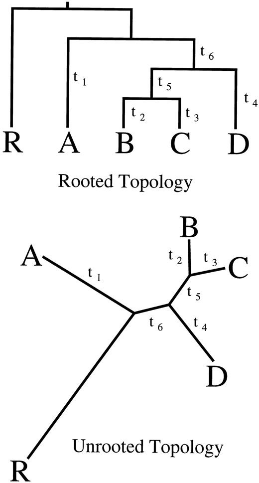
Fig. 1.—Topology used for simulation under a molecular clock. Taxon R is assigned as the outgroup (having diverged before the remaining taxa) to allow rooting at an arbitrary position along taxon R's branch

Open in new tabDownload slide

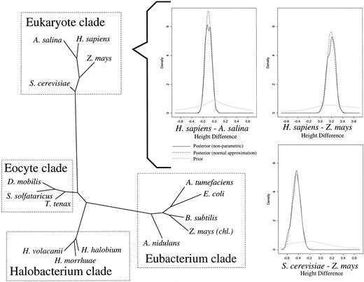
Fig. 2.—The Tree of Life modal (87% ± 3%) topology under TN93 (left). Branch lengths are drawn to scale. Plots of the marginal posterior (solid line), normal approximation to the posterior (dashed), and prior (dotted) for the three molecular-clock height differences (Δ_ij) within the Eukaryote clade are shown (right). The data do not support a molecular-clock restriction, as the posterior densities are less than the prior density at Δ_ij = 0

Open in new tabDownload slide

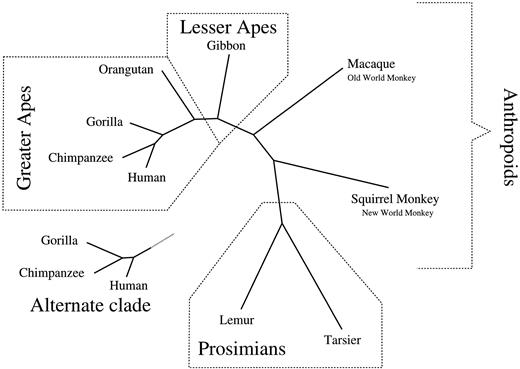
Fig. 3.—The two dominant topologies for primates under TN93 using one rate class. The complete displayed topology has a posterior probability of 90% ± 3%, while the alternate clade accounts for the remaining 10%. Branch lengths are drawn to scale

Open in new tabDownload slide

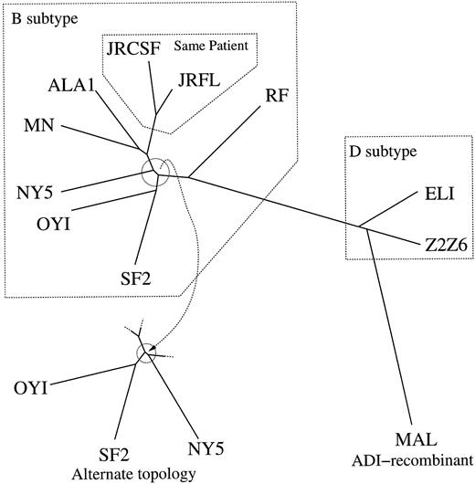
Fig. 4.—Two topologies account for 100% of the posterior for HIV under TN93. Branch lengths are drawn to scale. The two topologies converge as the circled internal branches approach zero

Open in new tabDownload slide

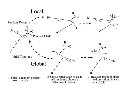
Fig. 5.—Local and global pendant leaf algorithms.

We thank James Lake for supplying the aligned sequences used in the TOL example and Karin Dorman and John Boscardin for their helpful criticism. M.A.S. was supported by a predoctoral fellowship from the Howard Hughes Medical Institute. J.S.S. was partially supported by USPHS grants AI28697 and CA16042.

literature cited