


Abstract
We consider three approaches for estimating the rates of nonsynonymous and synonymous changes at each site in a sequence alignment in order to identify sites under positive or negative selection: (1) a suite of fast likelihood-based “counting methods” that employ either a single most likely ancestral reconstruction, weighting across all possible ancestral reconstructions, or sampling from ancestral reconstructions; (2) a random effects likelihood (REL) approach, which models variation in nonsynonymous and synonymous rates across sites according to a predefined distribution, with the selection pressure at an individual site inferred using an empirical Bayes approach; and (3) a fixed effects likelihood (FEL) method that directly estimates nonsynonymous and synonymous substitution rates at each site. All three methods incorporate flexible models of nucleotide substitution bias and variation in both nonsynonymous and synonymous substitution rates across sites, facilitating the comparison between the methods. We demonstrate that the results obtained using these approaches show broad agreement in levels of Type I and Type II error and in estimates of substitution rates. Counting methods are well suited for large alignments, for which there is high power to detect positive and negative selection, but appear to underestimate the substitution rate. A REL approach, which is more computationally intensive than counting methods, has higher power than counting methods to detect selection in data sets of intermediate size but may suffer from higher rates of false positives for small data sets. A FEL approach appears to capture the pattern of rate variation better than counting methods or random effects models, does not suffer from as many false positives as random effects models for data sets comprising few sequences, and can be efficiently parallelized. Our results suggest that previously reported differences between results obtained by counting methods and random effects models arise due to a combination of the conservative nature of counting-based methods, the failure of current random effects models to allow for variation in synonymous substitution rates, and the naive application of random effects models to extremely sparse data sets. We demonstrate our methods on sequence data from the human immunodeficiency virus type 1 env and pol genes and simulated alignments.
Introduction
Determining the selection pressures that have shaped genetic variation forms a major part of many studies of molecular evolution. A common approach to this problem involves estimating the rates of nonsynonymous (dN) and synonymous (dS) substitutions. Estimates of dN significantly different from dS provide convincing evidence for nonneutral evolution. This approach is attractive as it does not make any assumptions regarding the demographic history of the population, unlike many “neutrality tests” (Tajima 1989, 1996; Fu and Li 1993a, 1993b; Deng and Fu 1996; Fu 1997; Misawa and Tajima 1997; Fay and Wu 2000), which compare estimates of effective population size obtained using different measures of genetic variation.
Initial studies of selection pressure relied upon the average dN/dS ratio for the region of interest, either using distance-based methods (Li, Wu, and Luo 1985; Nei and Gojobori 1986; Li 1993; Pamilo and Bianchi 1993; Comeron 1995; Yang and Nielsen 2000) or maximum likelihood methods (Goldman and Yang 1994; Muse and Gaut 1994); however, such approaches lack statistical power to detect positive selection as only a few sites may be under selection. Subsequently, methods have been proposed to study selection on a site-by-site basis. We classify these approaches into three classes: those that count the number of nonsynonymous and synonymous substitutions along the phylogeny (counting methods), those that assume a distribution of rates across sites and infer the rate at which individual sites evolve given this distribution (random effects models), and those that estimate the ratio of nonsynonymous to synonymous substitutions on a site-by-site basis (fixed effects models).
The first class, which we call counting methods, involves estimating the number of nonsynonymous and synonymous changes that have occurred at each codon throughout the evolutionary history of the sample. This approach was first proposed by Suzuki and Gojobori (1999) and involves reconstructing the ancestral sequences, for example, using parsimony (Suzuki and Gojobori 1999) or likelihood-based methods (Nielsen 2002; Nielsen and Huelsenbeck 2002; Suzuki 2004); the latter can take into account the uncertainty in the ancestral reconstructions. These methods are attractive as they are computationally fast and hence can be applied to large data sets and do not involve making any assumptions regarding the distribution of rates across sites. However, counting methods may lack power, especially for data sets comprising a small number of sequences or low divergence, as the power of the test is limited by the total number of inferred substitutions at a site. In addition, counting the number of changes between ancestral states may underestimate the true number of substitutions, and hence, the number of changes inferred using this approach may not accurately reflect the rate at which a site is evolving.
The second class of methods, originally described by Nielsen and Yang (1998), involves fitting a distribution of substitution rates across sites and then inferring the rate at which individual sites evolve. When this site-by-site inference is based on the maximum likelihood estimates of the rate parameters, this inference is known as empirical Bayes (Nielsen and Yang 1998; Yang et al. 2000), whereas when rate class assignments are based on the posterior distribution of rate parameters, this is known as a hierarchical Bayes approach (Huelsenbeck and Dyer 2004); the latter acknowledges that the rate distribution parameters are subject to error, whereas an empirical Bayes approach treats these parameters as known. Due to the computational complexity of the models and the concern that the use of prior distributions for parameters in a fully hierarchical Bayesian approach may unduly affect the results, most studies have employed an empirical Bayes approach to identifying sites under selection. When the assumed and the true distribution of rates are similar, we might expect that a random effects model will have more power to detect positive or negative selection than a fixed effects model or counting-based methods. However, for small data sets, the errors in estimation of the rate distribution may be large, such that empirical Bayes approaches may give misleading results, while a hierarchical Bayes approach may be very sensitive to prior assumptions of the distribution of rate parameters.
The third class of methods involves fitting substitution rates on a site-by-site basis. Such models are known as fixed effects in the statistical literature. These models can be considered as an extension of the model proposed by Yang and Swanson (2002), who considered two classes of sites specified a priori evolving under different dN/dS. Suzuki (2004) proposed a model in which the ratio of nonsynonymous to synonymous substitution rates was estimated for each codon using maximum likelihood and a likelihood ratio test (on one degree of freedom) was used to test whether this ratio was significantly different from 1. Like counting methods, fixed effects models make no assumption regarding the distribution of rates across sites. We might expect that such an approach would give a more accurate (less biased) representation of substitution rates at a site than counting methods. However, fixed effects models are typically slower than counting methods and may be difficult to fit due to the large number of parameters involved, as reported by Nielsen (1997) in the context of models of nucleotide substitution.
There has been much discussion of whether counting methods or random effects models are better approaches for the analysis of selection pressure (Suzuki and Nei 2001, 2002, 2004; Sorhannus 2003; Wong et al. 2004). However, a fair comparison between these approaches is not as straightforward as it might initially seem. First, counting-based methods implicitly allow for variable synonymous rates across sites, whereas the fixed effects model of Suzuki (2004) and the random effects models of Nielsen and Yang (1998) and Yang et al. (2000) assume that the synonymous substitution rate is the same for all sites. Yang and Swanson (2002) found that the inclusion of variable synonymous substitution rates between two classes of sites specified a priori gave a much better fit to data sets of abalone sperm lysin genes and human major histocompatibility complex class I genes. Second, in order to determine how the assumption of a rate distribution in a random effects model affects the results, it may be more appropriate to compare random effects models with fixed effects models, rather than compare random effects models with counting-based methods. Third, in order to compare between methods, they should ideally be based on the same underlying model of codon substitution.
We investigate the use of counting methods and random effects and fixed effects models for the detection of positive and negative selection at a site. Our counting method employs maximum likelihood ancestral reconstructions, unlike Suzuki and Gojobori (1999), who employed parsimony, and unlike Nielsen (2002) and Nielsen and Huelsenbeck (2002), who took a Bayesian approach. Suzuki (2004) proposed an ad hoc ancestral state reconstruction method, which first reconstructs amino acid ancestral states using an inefficient likelihood algorithm and then employs parsimony to map codon states restricted by amino acid inferences. A rigorous likelihood-based reconstruction performed in the codon-state space allows us to test the impact of uncertainty of ancestral reconstruction on the detection of sites under positive and negative selection without making prior assumptions regarding parameters such as branch lengths. Our random effects maximum likelihood model allows variation in both nonsynonymous and synonymous rates (cf. Nielsen and Yang 1998; Yang et al. 2000). Our fixed effects maximum likelihood approach also allows both nonsynonymous and synonymous substitution rates to vary on a site-by-site basis (cf. Suzuki 2004) without specifying site classes a priori (cf. Yang and Swanson 2002). All three approaches incorporate a general model of codon substitution, which allows us to rule out spurious results based on biased nucleotide frequencies. We present applications of our approaches to sequence data from the human immunodeficiency virus type 1 (HIV-1) env (envelope) and pol (polymerase) genes and conduct a series of simulations to assess the statistical properties of each testing approach.
Materials and Methods
Estimation of Phylogeny and Codon Substitution Model
Our implementations of counting, random effects, and fixed effects models are all based on an underlying phylogeny and codon substitution model, which permits a fair comparison between these approaches. In this section, we present a process by which an estimate of a phylogeny, codon frequencies, and substitution parameters and associated branch lengths can be obtained using a series of approximations to reduce the amount of computational effort.
Estimation of Phylogeny and Nucleotide Substitution Bias
We attempt to achieve a reasonable trade-off between the computational effort and the quality of the estimates of the phylogeny and a nucleotide substitution model using an iterative process. An initial estimate of the phylogeny is obtained by neighbor-joining (Saitou and Nei 1987) using the Tamura-Nei distance (Tamura and Nei 1993). Our simulations and applications to many data sets (not included in this paper) suggest that all the methods presented are robust to some errors in phylogenetic tree reconstruction, although a sensible effort to reconstruct a “good” phylogeny is always advisable.
Fitting of a Codon-Based Substitution Model
The MG class models differ from their GY (Goldman and Yang 1994) counterparts (used in Yang [1997], for instance) in that GY models use πy, i.e., the frequency of the target codon in place of
Model Fit and Approximation Quality
HIV-1 Envelope | HIV-1 AZT-Treated Reverse Transcriptase | HIV-1 Drug-Naive Reverse Transcriptase | |
|---|---|---|---|
| MG94 × REV | log L = −1,121.4 | log L = −5,941.21 | log L = −18,310.28 |
\({\hat{{\omega}}}{=}1.13{\,}(0.94,1.34)\) | \({\hat{{\omega}}}{=}0.19{\,}(0.17,0.21)\) | \({\hat{{\omega}}}{=}0.13{\,}(0.12,0.14)\) | |
| Selected model | Matrix: (001101) | Matrix: (010020) | Matrix: (012232) |
| log L = −1,126.47 | log L = −5,950.48 | log L = −18,333.4 | |
\({\hat{{\omega}}}{=}1.25{\,}(1.04,1.48)\) | \({\hat{{\omega}}}{=}0.19{\,}(0.17,0.21)\) | \({\hat{{\omega}}}{=}0.14{\,}(0.13,0.16)\) | |
| Approximate model | log L = −1,126.7 | log L = −5,959.09 | log L = −18,373.04 |
\({\hat{{\omega}}}{=}1.25{\,}(1.04,1.48)\) | \({\hat{{\omega}}}{=}0.20{\,}(0.18,0.22)\) | \({\hat{{\omega}}}{=}0.14{\,}(0.13,0.15)\) | |
| GY94 model | log L = −1,137.7 | log L = −6,004.5 | log L = −18,565.4 |
\({\hat{{\omega}}}{=}0.91\) | \({\hat{{\omega}}}{=}0.15\) | \({\hat{{\omega}}}{=}0.11\) | |
| Branch approximation | c = 0.971n + 0.0007 | c = 1.01n − 0.0001 | c = 1.02n − 0.0002 |
| r2 = 0.996 | r2 = 0.949 | r2 = 0.998 | |
| 99.99% CI | 99.99% CI | 99.99% CI | |
| SLAC comparison | PS: e = 0.998a − 0.002 | PS: e = a − 3 × 10⁻⁶ | PS: e = 0.996a − 0.004 |
| r2 = 0.996 | r2 = 1 | r2 = 0.9995 | |
| NS: e = 1.004a + 0.0004 | NS: e = 0.99997a + 7 × 10⁻⁶ | NS: e = 0.995a + 3 × 10⁻⁵ | |
| r2 = 0.995 | r2 = 1 | r2 = 0.9995 |
NOTE.—Estimates of ω are given together with their 95% profile likelihood confidence intervals (CI). The linear regressions use the following notations: c, branch length derived from a full fit using MG94 × REV codon model; n, branch length derived from fitting the selected nucleotide model; e, SLAC P value for dN > dS (PS) or dN < dS (NS) at a site derived from the full MG94 × REV model; and a, SLAC P value for dN > dS at a site derived from the approximate codon model.
Approximating Branch Lengths in a Codon Substitution Model
Fitting the entire codon model (ω, rate bias parameters and branch lengths) to large data sets is time consuming; thus, reasonable approximations are called for. The idea of approximating codon branch lengths with values derived from nucleotide models was previously investigated by Yang (2000), who found that there was a high degree of linear correlation between branch lengths derived from nucleotide models and those found with codon models but that nucleotide branch lengths appeared to be slightly shorter that those in codon models with rate variation. We estimated the length of a codon branch
Parameter space can be further reduced if nucleotide bias parameters Rij in the codon model are approximated with values from the best-fitting nucleotide model. This approximation may be affected by the fact that for data sets with high or low values of ω the sampling of different nucleotide substitutions may be seriously biased by the structure of the genetic code.
Testing the Validity of the Approximations
While the approximations described above may not hold in general, one can verify their validity, albeit at a rather steep computational cost. A more accurate phylogeny can be obtained by searching for phylogenies with a higher likelihood. Nucleotide substitution biases and branch lengths can be estimated using maximum likelihood within the context of a codon substitution model rather than a nucleotide substitution model. For the data sets utilized in this study, as well as many others that we have analyzed in other contexts, the approximations appear to be reasonable; the use of approximate branch lengths and nucleotide bias parameters does not result in a dramatic drop in model goodness of fit (as measured, for example, by inclusion of the approximation in the 99% confidence set around the MLE derived from the full model), and there is a strong linear correlation between the approximate and the maximum likelihood parameter estimates and P values for the various tests (table 1; single-likelihood ancestor counting [SLAC] results given; fixed effects likelihood [FEL] and random effects likelihood [REL] are similar and not included for brevity).
Counting Methods
Our counting method involves counting the number of nonsynonymous and synonymous changes and testing whether the number of nonsynonymous changes per nonsynonymous site (dN) is significantly different from the number of synonymous changes per synonymous site (dS).
Single-Likelihood Ancestor Counting
Given an estimate of the phylogeny (topology and branch lengths) and the codon-based substitution model, we wish to infer the number of changes that have occurred along the phylogeny. The simplest method involves reconstructing ancestral sequences using the joint likelihood reconstruction method in the codon-state space. Similar methods were first proposed for protein data by Yang, Kumar, and Nei (1995), and an efficient dynamic programming algorithm due to Sankoff (1975) was adapted to the context of phylogenetic likelihood by Pupko et al. (2000). This reconstruction strategy avoids most of the problems in the original Suzuki-Gojobori method by disallowing stop codons, recovering a unique state at each internal tree node, and fully incorporating synonymous and nonsynonymous substitution structure into ancestral state reconstruction. The computational cost of this method is comparable to that of a single likelihood function evaluation under the codon model and requires less than a minute even for large (200–300 sequence) data sets on a desktop computer.
Treating the reconstructed sequences as known, the number of nonsynonymous and synonymous substitutions per codon site as well as the average numbers of nonsynonymous and synonymous sites per alignment column are computed in the spirit of the Suzuki-Gojobori method. Our counting scheme differs in that we exclude stop codons, incorporate weighting of nucleotide substitution biases estimated from the data, and permit ambiguous codons in the data to be analyzed in one of two ways. First, they can be resolved into the most frequent codon. This is most appropriate when ambiguous codons may have arisen due to sequencing errors or when there are many ambiguous codons at a site. Second, the counts can be averaged over all possible codon states, weighting by the relative frequency of each state.
πn denotes the frequency of nucleotide n in the alignment, and scaling constants cj are chosen so that the sum of each row in the matrix product is equal to 1. The matrix B is a rescaled version of the “jump rate” matrix for the substitution process inferred from nucleotide sequence data.
Given any codon translation table, for each non–stop codon c = ijk, i,j,k ∈ {A,C,G,T}, we evaluate the quantities ESc and ENc which are analogous to the number of synonymous and nonsynonymous sites for codon c in the Suzuki-Gojobori method. To accomplish this, we consider all possible nine codons which can be reached from c with a single-nucleotide substitution, discard all those which are stop codons, and weigh the remaining ones with their relative probabilities, defined in B. ESc is then obtained as the sum of the weights of codons synonymous with c and, analogously, ENc—the sum of the weights of codons not synonymous with c.
Weighted Ancestor Counting
An alternative approach to counting nonsynonymous and synonymous substitutions for the maximum likelihood ancestral reconstruction is to compute expected values over possible ancestral state assignments
We observe that while the RLS of a branch labeling is similar in concept to the conditional probabilities of observing a character at an internal tree node (Yang, Kumar, and Nei 1995), the quantities computed here and the algorithm used are different.
We extend the definition of synonymous and nonsynonymous sites and observed substitutions for every branch b by taking the sum of these quantities for every possible branch labeling weighted by the RLS and employ these values for computing
Further details of the weighted ancestor counting (WAC) algorithm, demonstrating that it averages over all possible ancestral states, are given in Supplementary Material online.
Sampling Ancestral States
When it is desirable to estimate statistical properties of functions of ancestral states, for example, to check whether the mode (most likely ancestral state) is a reasonable approximation to the full distribution of ancestral states, conditional on the parameter estimates, we extend the sampling method of Nielsen (2002) to codon characters, sample from the distribution of character states at internal nodes, induced by their relative likelihood support, and tabulate quantities of interest to assess their distributional properties.
For completeness, we provide the outline of the algorithm. For an internal node n, define the quantity f(n,c)—the likelihood of observing the subtree “rooted” at n, given that the character at n is c, where c indexes all possible non–stop codons c. Note that all the f(n,c) can be evaluated in a single pass of the pruning algorithm (Felsenstein 1981). The sampling algorithm traverses the tree preorder, and samples character states at internal nodes as follows.
Root
All Other Internal Nodes
Testing for Positive or Negative Selection
Finally, dS and dN at site 𝒟s are defined by setting
We note that the extended binomial distribution is an approximation to the true distribution of nonsynonymous and synonymous under the hypothesis of neutrality (Durrett 2005). In the Supplementary Material, we compare P values derived using the extended binomial distribution with P values derived from simulating the null distribution (i.e., dN = dS), which shows a broad agreement (r2 = 0.81) for our data set of HIV reverse transcriptase sequences isolated from treatment naive individuals. Together with the broad agreement of the counting-based methods (employing the extended binomial distribution) with likelihood-based methods, these results suggest that the extended binomial is a useful approximation, although further studies of the conditions under which the approximation is warranted would clearly be beneficial.
Fixed Effects Likelihood
We treat all shared model parameters Φ (the tree topology, branch lengths, and nucleotide rate biases) as known, and hence, each branch of the phylogenetic tree provides a realization of the substitution process described by the two-parameter rate matrix MG94* × REV. Because the standard phylogenetic framework assumes independence of evolutionary processes between tree branches, if all the ancestral states in a standard unrooted bifurcating tree on N sequences were known, then there would be 2N − 3 independent realizations of the substitution process (not identically distributed because branch lengths are, in general, different). However, because we must weight over unknown ancestral states, the effective sample size will be smaller.
To test whether site s is under selection, we perform a likelihood ratio test by fitting a single parameter H0: αs = βs versus a two parameter HA: αs ≠ βs and employing the asymptotic
Although more computationally demanding than the counting-based methods described above, this approach trivially lends itself to parallelization: the fitting of each site can be performed independently of other sites. The computational cost of the FEL method grows linearly in the number of sequences and the number of unique alignment columns (patterns) in the data set. The method is sufficiently fast to be able to process gene-size alignments of several hundred sequences in a few hours on a small cluster of computers.
Random Effects Likelihood
We also compared the results of the heuristic counting-based methods and FEL described above with a random effects model, which allows rate variation in both nonsynonymous and synonymous rates and a general underlying nucleotide substitution model. Unlike the fixed effects model, the relatively small number of parameters in a random effects model permits simultaneous optimization of all parameters. We assume three classes of nonsynonymous rates and three classes of synonymous rates for the analyses presented here. We consider two measures for determining whether a site is under positive (or negative) selection: posterior probabilities (Nielsen and Yang 1998; Yang et al. 2000) and empirical Bayes factors, the ratio of posterior and prior odds of having ω > 1 (or <1) at a given site. All model parameters are held at their maximum likelihood estimates during the computation of posterior probabilities and Bayes factors.
While our random effects model is somewhat similar to the M3 (discrete categories) model of Yang et al. (2000), the major differences are the following.
(1) We explicitly allow both synonymous and nonsynonymous substitution rates to vary from site to site. Lack of this provision may lead to a high rate of false-positive results.
(2) We use a more general nucleotide substitution model. The use of a poor nucleotide substitution model may lead to some differences in the results; in any case, the computational cost of determining the best-fitting nucleotide model or fitting the MG94 × REV model is low.
(3) We model character frequency components of the rate matrix differently, which can give improved model fits.
In order to speed up the fitting of the full likelihood models with rate variation, we developed a simple scheme which allows the likelihood function to be distributed across multiple computer nodes (Kosakovsky Pond and Frost 2005). An additional speedup may be achieved by fixing branch lengths at values estimated by the nucleotide model as described previously and estimating only rate bias and distribution parameters. While offering an immense reduction in optimization times (more than 100-fold for very large data sets), the simplification does not seem to impact the conclusions of the method for our example data sets dramatically, although this may not hold in general for other data sets.
Sequence Data
In order to test our approaches, we consider three data sets of HIV-1 sequences of varying sizes. The first comprises 13 sequences of the C2-V5 region of the envelope gene (Leitner, Kumar, and Albert 1997; Leitner and Albert 1999), analyzed for positive selection in Yang et al. (2000). The second data set includes 81 subtype B sequences of the reverse transcriptase gene (positions 1–220) isolated from individuals treated with the azidothymidine (AZT) nucleoside reverse transcription inhibitor. The third data set includes 298 subtype B sequences of the reverse transcriptase gene (positions 1–220) isolated from untreated individuals. The last two data sets were obtained from the Stanford HIV Drug Resistance Database (http://hivdb.stanford.edu). Mutations present in only one sequence were replaced by the consensus (as these are likely to reflect sequencing errors), and identical sequences (matching ambiguous nucleotides) were removed from the alignment. Alignments and trees used in this study may be downloaded from http://www.hyphy.org/pubs/qnd.tgz.
Implementation
All sequence manipulations and analyses were performed with the HyPhy software package (Kosakovsky Pond, Frost, and Muse 2005). The parallel implementation of the rate variation models was run on an 18-processor Linux cluster. Additionally, a web-based interface to the SLAC, FEL, and REL methods running on a cluster of computers is available at http://www.datamonkey.org (Kosakovsky Pond and Frost 2005b).
Results
Statistical Properties of the Methods
We first conducted a series of simulations to assess the rates of false-positive (Type I) and false-negative (Type II) errors produced by each of the methods on various simulated data sets.
Recent results (Yang and Swanson 2002; Kosakovsky Pond and Frost 2005; Kosakovsky Pond and Muse 2005) suggest that many commonly analyzed sequences (HIV-1, hepatitis C, mammalian mitochondrial sequences, primate lysozyme) exhibit nontrivial site-to-site variation in synonymous substitution rates. Previous studies (Anisimova, Bielawski, and Yang 2001, 2002) have found that the likelihood approach of Nielsen and Yang performed well in the absence of synonymous rate variation; in this paper, we are primarily interested in the behavior of the methods when both synonymous and nonsynonymous rates vary from site to site. In the Supplementary Material, we provide an example of the relative performance of SLAC, FEL, REL, and Nielsen-Yang methods on a simulated alignment that does not include synonymous rate variation.
The methodology of Kosakovsky Pond and Muse (2005) allows one to test for the presence of synonymous rate variation in sequence data. Essentially, one fits the full REL model followed by a restricted REL model which does not allow for synonymous rate variation (similar to the M3 model of Yang et al. [2000]) and performs a likelihood ratio test. Because the models are nested, a χ2 approximation can be used to assess significance. In a later section we demonstrate that biological alignments of sufficient size analyzed in this manuscript support the model which allows synonymous rate variation.
Data Generation
We wanted to study the effects of the number of sequences in the alignment and the amount of sequence divergence on the performance of the methods. These parameters control how much information is available for inference at every site. We also examined the effect of using an incorrect topology and substitution model on the performance of the methods. Sequences were generated parametrically under an MG94 × REV model with the HyPhy (v0.99β) software package (Kovakovsky Pond, Frost, and Muse 2005). Substitution model parameters were set at RAC = 0.5, RAT = RCG = RGT = 0.25, RCT = 1.5, approximately based on estimates from HIV-1 pol alignments. Base frequencies used were those collected from an alignment of 55 subtype C HIV-1 reverse transcriptase sequences. We used symmetric bifurcating trees with 8, 16, 32, 64, or 128 tips, with branch lengths samples randomly from an exponential distribution with several different means λ such as 0.02 (e.g., single subtype HIV-1 pol trees), 0.15 (e.g., between-species primate mitochondrial DNA trees) and 0.5 (large divergence). Sequence length was set at 250 codons, which represents a fairly typical alignment length gathered from published selection analyses. Forty different data sets were simulated for each collection of parameter values (thus, at least 10,000 alignment sites were tested per set of simulation parameters). Because none of the methods can meaningfully infer selection at constant sites, such sites were excluded during result processing. All data employed for this study can be obtained from the http://www.hyphy.org/pubs/qnd_sims.tgz. HyPhy scripts used for simulations are available from the authors upon request (some require a message passing interface cluster environment cluster environment). Some of the simulation (32 sequence balanced trees) settings were similar to those reported as “difficult” for random effects models in Suzuki and Nei (2002).
Type I Errors
To determine the rates of Type I error (false positives) for detecting positively selected sites, we simulated data assuming neutrality (dN/dS = 1 at every site of the alignment) and analyzed them with SLAC, FEL, and REL methods. We note that this is (intentionally) a rather extreme case, and biological data sets are likely to exhibit rate variation, with many sites under purifying selection. In order to graphically compare the methods on the same scale (P values/posterior probabilities), we mapped Bayes factors (BF) for the REL method to a scale between 0 and 1 by 1/BF. In Supplementary Material (figs. 1–3), we show that the rates of Type I error in this scenario are well controlled by the nominal P value/posterior probability/Bayes factor in almost all scenarios. The counting methods appear to be susceptible to saturation effects of high sequence divergence and alignment size. This finding appears to contradict the claims made by Suzuki and Gojobori (1999), who found counting methods to always be conservative. This discrepancy is likely due to the fact that the original SG method could not handle highly variable sites, which are certain to arise in our simulation scenarios and contribute to inference errors and, possibly, to numerous differences in implementation details—for instance, parsimony-based ancestral sequence reconstruction can underestimate the number of substitutions at a site. Furthermore, counting methods remain conservative when sequence data exhibit rate variation, as demonstrated in the following section. It is worth noting that this simulation regime is the worst possible scenario for counting methods because they are likely to suffer from overfitting of synonymous rates at each site.
Power and Type II Errors
To determine the rate of Type II error (false negatives), as well as to assess the rate of Type I error in a more complex scenario, we simulated data sets with a rather complex pattern of site-to-site rate variation: both the baseline mutation rate and the strength of selection varied among sites. Specifically, each simulated alignment contained 375 codons with the following distribution of rates:
225 negatively selected sites: 75 codons with αs = 1/3 and βs = 1/30 (ωs = 0.1), 75 codons with αs = 1 and βs = 0.2 (ωs = 0.2), and 75 codons with αs = 3 and βs = 1.5 (ωs = 0.5);
75 neutral sites: 25 codons with αs = βs = 1/3, 25 codons with αs = βs = 1, and 25 codons with αs = βs = 3; and
75 positively selected sites: 25 codons with αs = 1/3 and βs = 4/3 (ωs = 4), 25 codons with αs = 1 and βs = 3 (ωs = 3), and 25 codons with αs = 3.0 and βs = 6.0 (ωs = 2).
In this scenario, there are three independent values for αs (1/3, 1, and 3) and seven independent values for βs (1/30, 0.2, 1/3, 4/3, 1.5, 3, and 6).
In order to fairly compare different methods with the same set of simulation parameters, we need to ensure that the Type I error rates are the same for the methods being compared. Setting nominal α-levels to the same threshold will not, in general, suffice for the rates of false positives to be the same. A simple way to resolve this predicament is to employ receiver operating characteristic (ROC) curves (cf. Green and Swets 1966), which map the proportion of misidentified sites (false positives) to the proportion of correctly identified sites (true positives), for all possible nominal α-levels (P values, posterior probabilities, or Bayes factors) of the test. In essence, ROC plots illustrate what would have happened had we been able to choose α-levels of each test optimally. When plotted in the same coordinates, a test whose ROC plot dominates all others is superior, because for a fixed rate of Type I errors, it is able to achieve maximal power among all tests on the data in question. However, for practical purposes, it is also important to examine the performance of the test with the critical level determined by its nominal P value, posterior probability, or Bayes factor. For comparative purposes, we also included results from the widely used M8 model (Yang et al. 2000) modified to use the MG94 × (012232) model; this model considers variation in nonsynonymous rates only as a mixture between a beta distribution and a point mass.
Relative Performance
ROC curves for various numbers of sequences suggest that SLAC, REL, and FEL perform comparably (ROC curves roughly overlap for both positively and negatively selected sites) and gain power with increased numbers of sequences (fig. 1). For sufficiently large data sets (64 sequences or more), even the fast, conservative SLAC method has excellent power (Supplementary Material). It is interesting to note that while REL gives similar or better performance than SLAC or FEL for the 16-, 32- and 64-sequence data set, it performs worse than SLAC or FEL for the small 8-sequence data set. Given that the only difference between REL and FEL is in the assumption of a rate distribution in the REL approach, it appears that the poorer performance of REL is due to errors in the estimation of the rate distribution influencing the inferred rates at individual sites. Note that the M8 model, which does not allow for the synonymous variation present in the data, performs progressively worse than other methods with increased numbers of sequences (especially noticeable for 64 sequences) because it assigns many of the sites with elevated rates (but dN/dS < 1) as positively selected more and more reliably (also see next section). For eight sequences, M8 performs about as well as all other approaches, probably because there is insufficient sequence data for synonymous rate variation to have a noticeable impact.
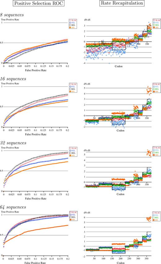
ROC curve mapping true positives versus false positives for detecting sites with dN > dS. Rates are recapitulated using average dN − dS at a site inferred by each of the methods. The reference gray line represents the true values of dN − dS. Symmetric trees with average branch length of 0.05 substitutions/site/unit time. Fifty replicates were analyzed for each setting.
Estimation of Rates
We considered the ability of each method to accurately estimate the difference in nonsynonymous and synonymous substitution rates at each site. For all three methods, SLAC, REL, and FEL, variation in the estimates was lower for larger data sets. Although all methods gave broadly similar estimates for substitution rates, SLAC tended to underestimate the substitution rates; FEL gave estimates of rates that were close to the true values, but with a lot of variation, especially for small data sets; and REL gave biased estimates of rates, but with less variation than FEL (fig. 1). For this scenario of rates, this is due to a combination of (1) the shrinkage of rate estimates toward the discrete rate categories assumed in the model and (2) the misspecification of the REL model—the simulated data were generated using a model that cannot be fully fitted using three categories of nonsynonymous rates. We have also analyzed simulated data in which the number of rate categories used to fit the data was the same as the number of categories used to generate the data; in this case, the REL model also gives biased estimates of rates due to shrinkage effects (results not shown). We note that, in general, we do not know the true distribution of substitution rates across sites. The M8 model of rate variation gave poor estimates of substitution rates due to failure to account for synonymous variation; sites evolving at high synonymous rates are falsely identified as having an elevated nonsynonymous rate.
Single-Likelihood Versus Weighted Ancestral Counting
We compared the estimated nonsynonymous and synonymous rates and associated P values (for dN < dS and dN > dS) for SLAC, which uses a single maximum likelihood reconstruction, and WAC, which weights over all possible reconstructions. Rate estimates and associated P values were extremely similar for the two approaches, suggesting that the use of a single reconstruction does not lead to biased results compared to weighting across all reconstructions, at least for the simulation scenario presented here, while requiring far less computational effort. For example, using an alignment on 32 sequences, false-positive (FP) and true-positive (TP) rates of detecting sites under positive selection (as functions of P values) exhibited excellent linear correlation: FPWAC = 0.986 × FPSLAC + 0.0003 (r2 = 0.997) and TPWAC = 1.031 × TPSLAC + 0.0002 (r2 = 0.998).
The Choice of Cutoff for Statistical Significance
For the SLAC and FEL methods, the rates of Type I and Type II errors for a given P value were rather similar (fig. 2), especially for large data sets, although both methods were conservative (Type I error much smaller than the nominal P value). For small data sets, SLAC was more conservative than FEL. REL appears to have false-positive rates similar to those stipulated by nominal α-levels (at least for small α-levels), regardless of whether they are based on mapped Bayes factors or posterior probabilities (fig. 2).
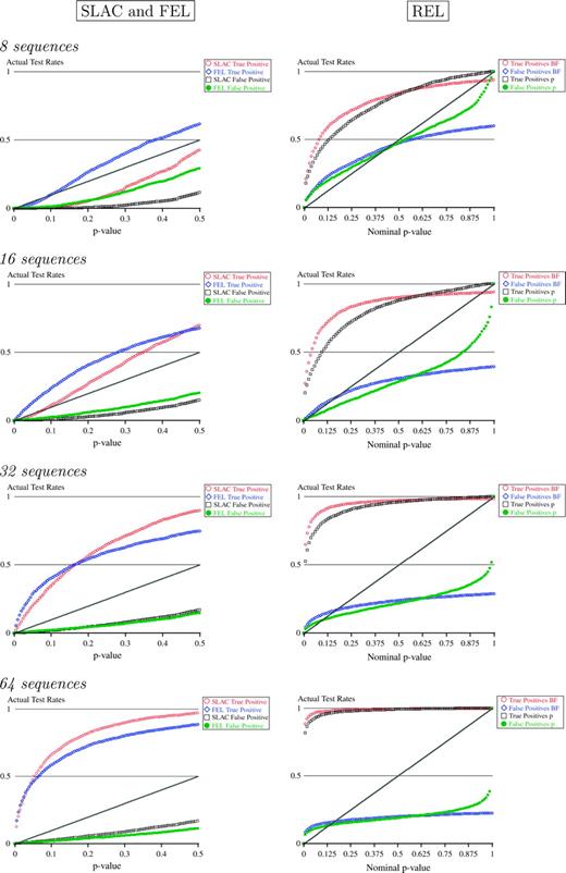
True- and false-positive rates as functions of nominal α-levels. P values were used for SLAC and FEL, and posterior probabilities and mapped Bayes factors were used for REL. Gray lines provide expected Type I error rates based on the α-level of the test.
Applications to Biological Data
We applied counting methods and fixed effects and random effects models to three biological data sets of HIV-1 sequences, comprising different numbers of sequences. We first obtained approximate estimates of the phylogeny and the patterns of nucleotide and codon substitution bias for each data set (table 1). For all three data sets, nonstandard models of nucleotide evolution were selected. Approximate branch lengths were extremely similar to maximum likelihood branch lengths (with correlation coefficients greater than 0.9), and the use of approximate branch lengths did not result in a large drop in goodness of fit as measured in terms of likelihood. The use of a GY model of codon substitution (Goldman and Yang 1994) resulted in a worse fit than an MG model of codon substitution (Muse and Gaut 1994) for all three data sets (table 1); hence, an MG model was used as a basis for our analyses.
HIV Envelope Sequences
We first considered a small data set consisting of 13 HIV-1 sequences of the viral envelope gene, each 91 codons long, analyzed by Leitner and coworkers (Leitner, Kumar, and Albert 1997; Leitner and Albert 1999), who found that the phylogenetic topology and branch lengths accurately recapitulated the known transmission history of HIV in these individuals. In Yang et al. (2000), many models of nonsynonymous rate variation were fitted to these data, and 3–10 sites were found to be under positive selection depending on the choice of the model.
Both SLAC and WAC yielded similar results for sites under selection (table 2), although inference at some highly variable sites appeared susceptible to uncertainties in ancestral state reconstruction. For example, at codon 28, which both SLAC and WAC identified as being under positive selection with P value of 0.12, the estimates of dN − dS and the P value for dN > dS had a large confidence interval based on 1,000 ancestral samples (table 2). At a significance level of 0.06, the FEL test also picked out this site as being under positive selection, with a higher estimate of dN − dS. In the REL method, synonymous rates αs and nonsynonymous rates βs were sampled from two independent general discrete distributions with two bins (estimated at Pr{αs = 0.0} = 0.55 and Pr{αs = 2.23} = 0.45) and three bins (estimated at Pr{βs = 0.0} = 0.29, Pr{βs = 1.04} = 0.54} and Pr{βs = 4.8} = 0.17), respectively, and all parameters, including branch lengths, were optimized. The test for synonymous rate variation was inconclusive with likelihood ratio test (LRT) just failing to reject the null of constant synonymous rates (P = 0.13), while Akaike's Information Criterion (AIC) barely chose the model with synonymous rate variation (2,251.36 vs. 2,251.48). Using a Bayes factor cutoff of 50, four sites (26, 28, 51, 66) were predicted to be under positive selection and 10 sites were predicted to be under negative selection. This Bayes factor cutoff corresponded to extremely high posterior probabilities (table 2). Using a posterior probability cutoff of 0.9, 11 sites were identified as being under positive selection and 13 sites were identified as being under negative selection. Due to small size of the alignment, we caution that P values of the tests should be treated as nominal.
Positively and Negatively Selected Sites in HIV-1 Envelope Data Identified by At Least One of the Methods
Counting Methods | Likelihood Methods | ||||||||
|---|---|---|---|---|---|---|---|---|---|
| Codon | SLAC | WAC | Sampler | FEL | REL | ||||
| 3 | −1.92 (0.30) | −1.92 (0.30) | −1.92:−1.92 (0.30:0.30) | −2.67 (0.11) | −1.98 (121.90; 0.9928) | ||||
| 4 | N | −2.05 (0.30) | −2.07 (0.30) | −2.05:−2.05 (0.30:0.30) | −5.73 (0.05) | −1.98 (216.54; 0.9959) | |||
| 13 | N | −7.45 (0.03) | −7.21 (0.03) | −9.53:−6.73 (0.01:0.03) | −23.70 (0.00) | −1.98 (315.29; 0.9972) | |||
| 20 | N | −6.26 (0.07) | −6.02 (0.08) | −6.26:−1.81 (0.07:0.45) | −18.95 (0.01) | −1.07 (39.56; 0.9782) | |||
| 26 | 3.78 (0.25) | 3.85 (0.24) | 3.10:4.46 (0.21:0.35) | 4.96 (0.20) | 4.08 (61.24; 0.9819) | ||||
| 28 | P | 6.06 (0.12) | 6.23 (0.12) | 5.86:8.03 (0.04:0.16) | 9.84 (0.06) | 4.08 (6,196.99; 0.9998) | |||
| 40 | −3.39 (0.31) | −2.67 (0.38) | −3.39:2.49 (0.31:0.73) | −10.00 (0.00) | 2.10 (10.06; 0.8988) | ||||
| 43 | −1.71 (0.33) | −1.71 (0.33) | −1.71:−1.71 (0.33:0.33) | −1.24 (0.16) | −1.98 (487.40; 0.9982) | ||||
| 45 | N | −2.56 (0.26) | −2.63 (0.26) | −4.27:−2.56 (0.11:0.26) | −8.30 (0.04) | −1.07 (59.48; 0.9854) | |||
| 47 | N | −3.09 (0.22) | −3.11 (0.22) | −3.09:−3.09 (0.22:0.22) | −7.50 (0.04) | −1.98 (148.32; 0.9941) | |||
| 51 | 4.27 (0.31) | 4.33 (0.31) | 4.20:5.04 (0.24:0.34) | 5.83 (0.22) | 4.08 (208.93; 0.9946) | ||||
| 61 | −3.83 (0.24) | −3.85 (0.24) | −3.83:−3.83 (0.24:0.24) | −1.92 (0.32) | −1.07 (110.90; 0.9921) | ||||
| 66 | 1.24 (0.57) | 2.61 (0.46) | −4.55:6.69 (0.11:0.90) | −8.14 (0.37) | 2.10 (335.13; 0.9966) | ||||
| 77 | N | −3.83 (0.16) | −3.85 (0.16) | −3.83:−3.83 (0.16:0.16) | −19.53 (0.02) | −1.98 (229.98; 0.9962) | |||
| 78 | N | −1.72 (0.39) | −1.72 (0.39) | −1.72:−1.72 (0.39:0.39) | −4.74 (0.08) | −1.98 (55.37; 0.9843) | |||
| 89 | N | −3.13 (0.18) | −3.14 (0.18) | −3.13:−3.13 (0.18:0.18) | −6.95 (0.03) | −1.98 (153.68; 0.9943) | |||
NOTE.—The first number for every method is an appropriately scaled dN − dS, so that they are directly comparable. The number in parentheses show P values for the appropriate test and the Bayes factor values for the REL method; posterior probabilities are also included for reference purposes, although they are not used in site classification. The entries for the Sampler method show 95% quantiles for the distribution of dN − dS and appropriate P values based on 1,000 ancestral samples. When a test is significant, the corresponding cell entry is given in bold. The letter next to the codon number represents consensus identification (“P” for positive and “N” for negative).
A possible difference between REL and the other two approaches is that when identifying the rates at individual sites using an empirical Bayes method, the parameters of the rate distribution are treated as known. As we demonstrate in the Supplementary Material, this effect can be dramatic and can account for most of the differences among the methods for this small data set.
HIV-1 pol Sequences
As an example of an intermediate size data set, we analyzed an alignment of 81 sequences of part of the HIV-1 pol gene which encodes reverse transcriptase. These sequences were isolated from virus from individuals who had been treated with the reverse transcriptase inhibitor AZT; hence, genetic variation in these genes is likely to reflect selection for drug resistance.
Two of the three classes of methods agreed on seven sites (35, 64, 69, 200, 207, 211, 215) under positive selection (table 2 in Supplementary Material). Of these, mutations at site 215 are known to confer strong resistance to AZT (Larder and Kemp 1989) and mutations at position 69 are known to contribute to AZT resistance in combination with mutations at other sites (Fitzgibbon et al. 1991; Winters and Merigan 2001). The REL method predicted the largest number of sites (11) to be positively selected, including all but one of those found by other methods. The hypothesis of constant synonymous rates was rejected both by LRT (P≪0.001) and AIC (11,316.1 vs. 11,392.3). A larger data set also led to reduced relative errors both in distribution parameters and ancestral state estimates when compared to the small HIV-1 envelope data set. This observation is consistent with the much better agreement between likelihood and counting methods than in the previous example.
When scaled to represent the expected number of nucleotide substitutions per codon site, dN – dS estimated by all the methods at putative positively selected sites were quite similar, with especially good agreement at the sites where all methods also inferred statistically significant dN − dS > 0 (table 1 in Supplementary Material). In contrast, the M8 model, in addition to having a much lower likelihood than the REL model that included synonymous variation, disagreed with the other methods at a number of sites that exhibited high numbers of synonymous changes. The M8 model classified position 70, for example, as one of the 7.3% of sites under selection (dN/dS = 1.87), with a high posterior probability (0.997) and Bayes factor (4,048). However, based on a maximum likelihood reconstruction, this site had a high number of synonymous changes (6), compared to 12 nonsynonymous changes. When scaled by the number of synonymous and nonsynonymous sites at this position, SLAC gave an estimate of dN − dS = −0.97 (P value for dN − dS > 0 = 0.77). FEL gave similar results, with an estimate of dN − dS = −4.75, with a P value for negative selection of 0.18. Our REL model estimated dN − dS to be −1.5, with a posterior probability of only 0.27 and a Bayes factor of only 3 for dN − dS > 0. While the estimate of dN − dS at an individual site varies by SLAC, FEL, and REL method, all methods agree that there is insignificant evidence for positive or negative selection at this site, whereas the M8 model, by failing to account for the high synonymous substitution rate at this position, concludes that there is extremely strong evidence for positive selection.
HIV-1 Drug Naive pol Sequences
For the final example, we chose a large data set with 297 sequences of part of the HIV-1 pol gene which encodes reverse transcriptase. These sequences were isolated from virus from individuals who had not taken reverse transcriptase inhibitors; hence, genetic variation in these genes is likely to reflect selection from the cellular immune response, rather than antiviral drugs. The hypothesis of constant synonymous rates for this alignment was rejected both by LRT (P≪0.001) and AIC (34,917.0 vs. 35,371.1).
Two out of three methods concurred in predicting seven (35, 135, 177, 200, 202, 211, 215) sites as positively selected (table 2 in Supplementary Material), three of which (35, 200, 211) were also found to be under selection in the first reverse transcriptase alignment. REL predicted the most (15) number of positively selected sites. We observe that at many of these sites, both SLAC and FEL approached significance, and given their somewhat conservative nature, they are likely to agree with REL if more sequences were available. REL, on the other hand, may be susceptible to increased shrinkage effects if the assumed and the true distribution of rates are in poor agreement.
Discussion
We have presented an exposition of detecting positive selection on sites in a sequence alignment using counting methods and maximum likelihood models which treat rate variation as either fixed or random effects. By basing counting-based methods on ancestral reconstruction using a codon-based substitution model, close comparisons can be made between fast heuristic methods and slower maximum likelihood–based methods. Simulation studies suggest that all three methods presented have well-controlled error rates, and by running a more computationally complex method on data sets of small or moderate sizes more power can be gained. We found it encouraging that, given sufficient biological data, all methods arrived at very similar conclusions, both on real and simulated data, and the main difference in the methods appears to lie in the conservative or liberal nature of the test statistic. When we accounted for this difference, using ROC curves, the performance of all methods on simulated data was virtually identical.
Failure to model variation both in synonymous and nonsynonymous substitution rates can, under some scenarios, lead to misleading results and should be avoided unless constancy of synonymous rates can be ascertained. All methods presented in this paper are able to adequately model such variation, whereas current implementations of fixed effects (Suzuki 2004) and random effects (Nielsen and Yang 1998; Yang et al. 2000) approach do not. If synonymous substitution rates are constant across sites, then site-by-site methods such as SLAC and FEL lack power compared to random effects approaches. We note that our REL method, which can incorporate synonymous substitution rate variation, still performs well in this scenario as the distribution of synonymous rates is estimated to be approximately uniform across the sequence alignment.
Failure to take biases in the underlying substitution process into account can result in altered estimates of nonsynonymous and synonymous substitution rates. Additionally, it is possible that none of the “named” models adequately describe the evolution of a particular organism, and thus, nonstandard models should be considered. The impact of choosing an incorrect model of the underlying nucleotide substitution process can have a small, but detectable, effect on the power to detect selected sites.
Having made simplifying assumptions for all methods, such as using approximate branch lengths and rough phylogenies, we were able to dramatically reduce computational effort involved in the methods, without a significant sacrifice in goodness of fit. These simplifications are not essential to the methods and can be removed in favor of more accurate, albeit more time-consuming, approaches.
To determine the robustness of counting-based methods to the use of a single ancestral reconstruction, as was originally proposed in Suzuki and Gojobori (1999), we implemented two algorithms which take the uncertainty in ancestral reconstructions into account; the first averages over all possible reconstructions, while the second samples from all possible reconstructions. We found that inferences based on a single most likely ancestral reconstruction gave results extremely similar to those based on weighting over possible reconstructions at a much lower computational cost. For smaller data sets, the uncertainty in the number of changes that have occurred at a site can be substantial. This can result in results from single or weighted ancestral constructions being either too liberal or conservative depending on the structure of the data; for small data sets, it may be advisable to run a sampling-based approach in order to assess how uncertainty in reconstructions affects the results. For large data sets, the results of the three different counting methods appear to converge, at least for the data sets studied in this paper and based on simulation results. We recommend SLAC for data sets that are large (over 40 sequences) as SLAC is a very fast method, and the conservative nature of the test suggested by our simulations of nonneutral data is mitigated by its application to large data sets. Moreover, the speed of counting methods makes it possible to perform extensive Type I and Type II error simulations in the time it would take to perform a single fit of a random effects model.
Differences between empirical Bayes and counting-based methods of estimating substitution rates at a site may arise due to errors associated with estimation of the rate distribution. These errors are likely be substantial, especially for small data sets, as shown by wide profile likelihood intervals, and can result in large numbers of falsely positive inferences of selected sites (Supplementary Material), especially when using posterior probabilities rather than Bayes factors to infer positive selection. In such cases, a hierarchical Bayesian approach (Nielsen and Huelsenbeck 2002) may be more appropriate, but care must be taken in order that the results are not overly influenced by the choice of prior distribution on the rate parameters. For intermediate data sets (20–40 sequences), we recommend the use of our FEL method; by estimating the rates of nonsynonymous and synonymous substitution at each site directly, the need to assess errors in the underlying distribution of rates across sites is avoided, together with a performance advantage over REL in terms of speed and over SLAC in terms of power as a function of the nominal α-level of the test.
Our results contribute to the discussion of whether counting-based methods or random effects models are preferable in the identification of sites under positive or negative selection (Suzuki and Nei 2001, 2002, 2004; Sorhannus 2003; Wong et al. 2004). Our results suggest that differences between the counting method of Suzuki and Gojobori (1999) and the models of Yang et al. (2000) may arise due to a number of factors: (1) the highly conservative nature of counting-based methods, (2) the failure of previous random effects models to incorporate synonymous rate variation, (3) misspecification of the rate distribution in a random effects model, and (4) the failure to explore the sensitivity of results obtained using an empirical Bayes approach to errors in the estimation of the parameters of the rate distribution. With the exception of the extent to which the test statistic (P values, Bayes factors, or posterior probability) is conservative or liberal, counting-based methods and random effects methods give broadly similar results when both approaches allow synonymous variation and are applied to data sets of sufficient size. For small data sets, disagreement between counting, fixed effects, and random effects models seems inevitable. We find it difficult to make a definitive recommendation when only a few sequences are available for analysis. The conservative nature of counting and fixed effects methods may result in the lack of power to detect selection, while excessive errors in parameter estimates employed in empirical Bayesian analysis can lead to large Type I error rates. An application of all three methods, with high (e.g., 0.25) nominal α-levels for SLAC and FEL, followed by the classification of sites based on the consensus of the methods, coupled with analyses of simulated data, seems to be a reasonable approach to rule out spurious results.
Robin Bush, Associate Editor
We would like to express our thanks to Professor Andrew J. Leigh Brown (University of Edinburgh) for discussion and two anonymous reviewers for constructive criticisms. This research was supported by the National Institutes of Health (AI47745, AI43638, and AI57167), the University of California Universitywide AIDS Research Program (grant number IS02-SD-701), and a University of California, San Diego Center for AIDS Research/NIAID Developmental Award to S.D.W.F. (AI36214).
References
Anisimova, M., J. P. Bielawski, and Z. Yang.
———.
Comeron, J. M.
Deng, H. W., and Y. X. Fu.
Durrett, R.
Fay, J. C., and C. I. Wu.
Felsenstein, J.
Fitzgibbon, J., R. Howell, T. Schwartzer, D. Gocke, and D. Dubin.
Fu, Y. X.
Fu, Y. X., and W. H. Li.
Goldman, N., and Z. H. Yang.
Green, D. M., and J. A. Swets.
Huelsenbeck, J. P., and K. A. Dyer.
Huelsenbeck, J. P., B. Larget, and M. E. Alfaro.
Kosakovsky Pond, S. L., and S. D. W. Frost.
Kosakovsky Pond S. L., and S. D. W. Frost.
Kosakovsky Pond, S. L., and S. V. Muse.
Kosakovsky Pond, S. L., S. D. W. Frost, and S. V. Muse.
Lanave, C., G. Preparata, C. Saccone, and G. Serio.
Larder, B., and S. Kemp.
Leitner, T., and J. Albert.
Leitner, T., S. Kumar, and J. Albert.
Li, W. H.
Li, W. H., C. I. Wu, and C. C. Luo.
Misawa, K., and F. Tajima.
Muse, S. V.
Muse, S. V., and B. S. Gaut.
Nei, M., and T. Gojobori.
Nielsen, R.
Nielsen, R., and J. Huelsenbeck.
Nielsen, R., and Z. H. Yang.
Pagel, M.
Pamilo, P., and N. O. Bianchi.
Pupko, T., I. Pe'er, R. Shamir, and D. Graur.
Rodriguez, F., J. L. Oliver, A. Marin, and J. R. Medina.
Saitou, N., and M. Nei.
Sorhannus, U.
Suzuki, Y.
Suzuki, Y., and T. Gojobori.
Suzuki, Y., and M. Nei.
———.
———.
Tajima, F.
———.
Tamura, K., and M. Nei.
Tavaré, S.
Winters, M., and T. Merigan.
Wong, W. S. W., Z. Yang, N. Goldman, and R. Nielsen.
Yang, Z.
Yang, Z., S. Kumar, and M. Nei.
Yang, Z., and W. Swanson.
Yang, Z. H.
Yang, Z. H., and R. Nielsen.
