
Abstract
A better understanding of the various patterns in the coronavirus disease 2019 (COVID-19) spread in different parts of the world is crucial to its prevention and control. Motivated by the celebrated GLEaM model (Balcan et al., 2010[1]), this paper proposes a stochastic dynamic model to depict the evolution of COVID-19. The model allows spatial and temporal heterogeneity of transmission parameters and involves transportation between regions. Based on the proposed model, this paper also designs a two-step procedure for parameter inference, which utilizes the correlation between regions through a prior distribution that imposes graph Laplacian regularization on transmission parameters. Experiments on simulated data and real-world data in China and Europe indicate that the proposed model achieves higher accuracy in predicting the newly confirmed cases than baseline models.
1 Introduction
The outbreak of coronavirus disease 2019 (COVID-19) has impacted all aspects of the world significantly for a long. As of 26 Oct 2021, there have been over 243 million confirmed cases of COVID-19, including over 4 million deaths ([2]). Therefore, it is essential to study the spread of COVID-19 for better prediction and prevention of the disease. This paper first proposes a stochastic dynamical model that describes the spread of COVID-19 in multiple regions and then develops an algorithm to estimate the transmission parameters and their posterior distributions.
The model proposed in this paper is inspired by The Global Epidemic and Mobility (GLEaM) model proposed in [1]. GLEaM is a stochastic dynamic model to depict the spread of epidemics, integrating multiple data layers that couple metapopulations at the global level. The model involves 3362 subpopulations in 220 countries obtained from Voronoi tessellation, centered around major airports. These subpopulations are connected by a multi-layer mobility network composed of processes from short-range communication in geographically close subpopulations to international flights. In each subpopulation, the transmission of epidemics is modeled by a Susceptible-Exposed-Infected-Removed (SEIR) compartmental model that integrates short-range communication. After specifying the compartmental model and initial conditions, GLEaM can be run repeatedly to build a statistical ensemble for each point in the space of parameters, which can be further utilized for Monte Carlo analysis of epidemic parameters.
In the vast majority of GLEaM’s applications ([3, 4, 5, 6, 7, 8, 9, 10]), the parameters are estimated based on [11]. [11] performed the maximal likelihood analysis of the reproduction number R0 in the seed region Mexico. For each value of R0, the method generated the distribution of arrival time of the influenza A(H1N1) in 12 countries produced by 2 × 10³ GLEaM simulations. Then, the optimal R0 was chosen by maximizing the likelihood function of arrival time. [11] and subsequent works following its settings ([3, 4, 5, 6, 7, 8, 9, 10]) assumed that the epidemic was seeded from one region and the transmission parameters or the other parameters (like the introduction date and location) were estimated through the maximal likelihood analysis of arrival time or other events. In particular, the method in [11] was adopted in [5] to estimate the posterior distribution of R0 of COVID-19, which was assumed to be uniform for all subpopulations at all times. However, this setting is not suitable for the current scenario of the COVID-19 pandemic, since COVID-19 has lasted for a long time, and the community transmission has been widespread in most countries in the world [12]. To model the spread of COVID-19, both spatial and temporal heterogeneity of the transmission parameters are needed instead of directly modeling R0 as a periodic function of time as in [11], since the social behaviors, containment measures, medical conditions, and other elements that might have effects on the spread of COVID-19 may vary among different countries and over time.
Recently, [13] improved the model described above by estimating the initially infected individuals in each subpopulation through microblogging data from Twitter and also estimating the reproduction number R0 for USA, Italy, and Spain separately. Therefore, the method used in [13] involved spatial heterogeneity. However, in this study, international travel was not considered, and GLEaM was applied to each of the aforementioned countries (as an isolated system) independently. The transmission rates in all subpopulations of these countries were again presumed to be homogeneous. Furthermore, [13] also assumed that the initially infected individuals for each subpopulation were proportional to the total number of Twitter users in that subpopulation. Thus it still assumed that the severity of the pandemic at the initial outbreak of COVID-19 was uniform over the country, which is not the case for COVID-19.
In addition to the issues mentioned above, other potential concerns exist when using GLEaM to model the spread of COVID-19. As mentioned in the last section of [14], GLEaM can be used to simulate the spread of the epidemic under normal conditions since it uses the “steady-state” mobility data around the world. However, since the outbreak of COVID-19, the social order has been disrupted, and travel has been restricted in most countries. Thus GLEaM might not work well with its multi-layer mobility networks. Furthermore, the estimation of parameters using GLEaM is based on a large number of simulations to explore the space of parameters, which usually takes much computational time ([1]). In addition, although the social behavior, medical conditions, and other factors that affect the spread of COVID-19 may vary among different regions, these factors for regions that are geographically close or have similarities in other aspects still bear some resemblance. Hence, the transmission rates for COVID-19 should not only own heterogeneity but also correlate with each other. However, neither of the features is reflected in GLEaM or most of its applications.
As the consequences of the possible constraints of GLEaM described above, most of the papers using GLEaM to model the epidemics focus on estimating the transmission parameter in the “seed region” and mainly use the epidemic data at the beginning of the outbreak. However, since factors like government policies and social behavior result in spatial and temporal heterogeneity of the long-lasting spread of COVID-19 around the world, GLEaM and inference methods based on a large number of simulations using GLEaM may not be directly applied to estimate the transmission parameters of COVID-19 in different regions and periods.
In this paper, we propose a model inspired by the GLEaM framework that further enables both spatial and temporal heterogeneity of parameters, making it possible to model the ongoing spread of COVID-19 instead of only the initial outbreak as considered in most applications of GLEaM. Motivated by GLEaM, we include inter-district mobility in the model when such mobility data are available. For the inference of the parameters, we introduce an optimization algorithm that utilizes the correlation between districts. Furthermore, the posterior distribution of parameters is estimated by Markov chain Monte Carlo (MCMC) sampling starting from an optimal choice of the parameters obtained from the optimization process. This takes a much shorter time than the methods based on GLEaM simulations.
The main contributions of our paper are:
We propose a stochastic model to describe the epidemic’s lasting spread, allowing spatial and temporal heterogeneity of transmission parameters and transportation between districts.
Based on the model, we also design an algorithm that first makes inference for the parameters through a two-step procedure combining the information of correlation between districts, which is equivalent to imposing graph Laplacian regularization on the transmission parameters. Then, the algorithm estimates the posterior distribution efficiently by MCMC sampling with the estimated parameters as the initial points.
We compare the performance of the proposed model with the baseline models on both simulated data and real-world data.
- For the simulated data, the results show that combining heterogeneity and transportation into the model helps improve the performance of trajectory prediction and parameter estimation. Moreover, our inference algorithm that integrates the correlation of districts leads to further improvement in predicting the future trajectories.
- For the real-world data in China and Europe, the proposed model still outperforms the baselines in trajectory prediction.
Data sets used in this paper are publicly available. Our work focuses on proposing a new method for parameter inference and, consequently, answering questions regarding the long-lasting spread of COVID-19 in multiple regions.
A strength of the proposed model resides in introducing spatial and temporal heterogeneity of transmission parameters. We remark that there exist recent works which also involved different levels of heterogeneity in their models in various ways. [15, 16] utilized randomness in reproduction number to reflect heterogeneity of the population, using plate model with Bayesian method and heterogeneous well-mixed theory [17] with age-of-infection method [18], respectively. In addition, [19, 20, 21, 22, 23] adapted SEIR / Susceptible-Exposed-Infected (SEI) / Susceptible-Infected (SI) compartmental models similar to this paper. Among these works, [19, 20, 21] considered heterogeneity in the aspects of age groups, social links, and vaccination status separately. [22, 23], including spatial heterogeneity in one county and among states respectively, bore more similarity with this paper since they also allowed transmission parameters to be spatially heterogeneous and involved transportation between different regions. However, [22] only considered intracounty data, and the transportation was used to compute the effective size of compartments and did not affect the dynamic model. Furthermore, the transmission rates in [22] were determined by an SDE whose parameters were to be fitted. Therefore, [22] focused on a different scope from this paper. The settings of compartments in [23] are more realistic than the one considered in this paper by considering reporting rates. Nevertheless, compared with the model and inference algorithm described in Section 2, transmission rates in [23] were kept constant over time and were estimated using independent non-informative prior. Both [22] and [23] used Ensemble Kalman Filter, which samples particles in the state space according to the prior distribution and obtains the posterior distribution in the process of moving particles at each time step. This may be computationally less efficient than directly applying MCMC according to the posterior distribution with the initial point maximizing the likelihood function, as implemented in this paper.
The rest of the paper is structured as below. In Section 2, we introduce the stochastic dynamic model and corresponding inference algorithm. In Section 3, we compare the performance of trajectory prediction and parameter estimation of models with or without mobility, heterogeneity, or using correlation information in the inference part for the simulated data. Section 4 describes the real-world data used in this paper, presents the results and findings of applying our model to the COVID-19 data in China and Europe. We discuss our limitations and possible extensions in Section 5.
2 Method
2.1 Model Description
Motivated by the stochastic dynamic process constructed in [24], we propose a stochastic model that considers mobility.
Suppose there are n regions (region 1, …, n), and we consider the evolution of the epidemic within a period of T days (day 1, …, T). For each region, we consider the following epidemiology compartments:
Sk(t): Susceptible.
Ek(t): Exposed and infectious.
Hk(t): Hospitalized.
Rk(t): Recovered or dead.
The subscript k of the states denotes that they belong to the k-th region, and dependence on the continuous time t is addressed through expressing the states as functions of t ∈ [0, T ].
We also denote Nk(t) = Sk(t) + Ek(t) + Hk(t) + Rk(t) as the total population in the k-th region at time t. Nk(t) is allowed to be time-varying since the inter-region mobility is taken into consideration, especially for the days before the implementation of travel restrictions. In this report, we assume that  keeps constant over time. We also denote (Na)k(t) = Sk(t) + Ek(t) + Rk(t) as the total population that are permitted to move in the k-th region, excluding the hospitalized ones.
Furthermore, denote  as the traveling volume from region i to j on the t-th day (t = 1, …, T). Then the traveling matrix Wt on the t-th day can be written as
 Then, the transition dynamic of ξ(t) = {S1(t), E1(t), H1(t), R1(t), …, Sn(t), En(t), Hn(t), Rn(t)} ∈ {0, 1, 2, …, N }4n over t ∈ [0, T ] is described below:
Transmission in the k-th region: A case from Ek(t) chooses an individual from Nk(t) randomly at Poisson rate λk(t), and the individual chosen is infected if it is of state Sk(t). Note that this is different from traditional SEIR models, since we assume that for the COVID-19 case, the pre-symptomatic patients from Ek(t) can be contagious.
Hospitalization in the k-th region: Each individual in Ek(t) will be hospitalized with Poisson rate δ.
Recovery or death in the k-th region: Each individual in Hk(t) will transfer into Rk(t) with Poisson rate γk. The recovery rate γk owns spatial heterogeneity due to the uneven distribution of medical resources.
Transportation between regions: At the end of the t-th day, all the individuals in region i except the ones in Hi(t) have the same probability to travel from the i region to the j region, and the total traveling volume from the i region to the j region is
 . Thus, if we denote as the number of people transported from {Si(t), Ei(t), Ri(t)} to {Sj(t), Ej(t), Rj(t)} at the end of the t-th day, then follows a multinomial distribution. Specifically,
with .
. Thus, if we denote as the number of people transported from {Si(t), Ei(t), Ri(t)} to {Sj(t), Ej(t), Rj(t)} at the end of the t-th day, then follows a multinomial distribution. Specifically,
with .


For clarification, we list all the notations and the parameters in Table 1 below.
List of notations and parameters
Now we consider the mean-field differential equation system in (2.3) ([25, 26]), which is a deterministic version of the stochastic model above:
 where
where  is the deterministic counterpart of Sk(t) and so on, and (Ca)k(t) and (Ra)k(t) are the accumulated confirmed cases and the accumulated removed cases determined by the ordinary differential equation (ODE) system (2.3) in the k-th region at time t, respectively.
Among the compartments in (2.3),  and
and  can actually be observed, whose observed counterparts are denoted as
  and
and  , respectively.
For inference of parameters, we further denote (ΔCa)k(i) = (Ca)k(i) − (Ca)k(i − 1) as the newly confirmed cases on the i-th day (k = 1, …, n, i = 2, …, T), and  as the observable counterparts of (ΔCa)k(i). The same convention holds for the definitions of (ΔRa)k(i) and
  .
.
For the remaining latent variables, Rk(0) is assumed to be 0, while Ek(0) and Hk(0) are left to be inferred for each k = 1, …, n.
Note that in contrast to the work based on GLEaM [11, 3, 4, 5, 14], we allow parameters to possess both spatial and temporal heterogeneity. Moreover, the transportation between regions is also considered in the model when the traveling matrix Wt is available, which is similar to GLEaM.
We finally emphasize that the model and the inference algorithm described below can be applied when the newly confirmed and recovered cases, the transportation matrix in each day, and the timeline of significant policy responses to the pandemic are available.
2.2 Estimation of Model Parameters
A two-step procedure of estimating parameters is described below.
First, note that δ, the inverse of the average time for a person from being exposed to hospitalized, is prefixed to be δ = 0.14 for all regions and all time. According to [27], the mean duration of incubation period is 5.2 days. Furthermore, we assume that the average time for an individual from showing symptoms to being hospitalized is 2 days for simplicity. Thus, the mean duration for an individual from being exposed to being hospitalized is 7.2 days, whose inverse value is approximately 0.14.
Thus, the model parameters that need to be estimated are  .
.
A two-step analysis is adapted for the estimation. We first make inference for  utilizing the newly recovered cases and the accumulated hospitalized cases. After the estimation of
  are then estimated by maximizing the posterior distribution, where we introduce a prior distribution combining the information of correlation between regions. In addition, the marginal posterior distributions of
  can also be obtained by running MCMC sampling starting from the optimizer
  of the posterior distribution. Then we complete the inference of
  .
.
Mathematically, given parameters Θ, we can run the ODE system (2.3) on [0, T ] and denote  as the values determined by (2.3) on the i-th day, and
  as the observed counterpart of xi.
Step 1: Estimate

We first estimate  by maximizing
  over γk for each k. By assuming that the newly recovered cases in one day follow a Poisson distribution whose mean equals to the product of γk and the accumulated hospitalized cases (which is the difference between the accumulated confirmed cases and the accumulated recovered cases, and thus is observable) the day before, we have that
 Then, we estimate
  for each k separately.
Step 2: Estimate and the marginal posterior distributions of


Next, we estimate the remaining parameters  as follows.
First, note that λk is the transmission rate, which reflects the infectivity of the virus, the prevention and control measures, and the rates of close contacts in the k-th region. In this report, λk is allowed to be time-varying. Specifically, the total T days are split into two periods with time thresholds Tk chosen for each k = 1, …, n, then λk = λk,1 if t < Tk and λk = λk,2 otherwise.
Notice that the ODE system (2.3) is the mean-field version of our stochastic model, and  (especially {(ΔCa)k(i)}k,i) are determined by the parameters, thus by the Markov property,
  are all independent for k = 1, …, n, i = 1, …, T conditioned on the parameters
  . Furthermore we suppose that
  . Thus, the likelihood of
  can be written as
 Now, we denote the posterior distribution of
  as
as  . Then by Baysian formula,
 where
where  is the prior distribution of
  to be determined and
  is a constant irrelevant to
  . We further denote
  , then
 To fit the realistic evolution of the epidemic more precisely,
  is estimated as
  with reasonable prior distribution
  . Then, MCMC sampling scheme starting from
  is applied to get the posterior distribution for
  . This process might possess higher computational efficiency than choosing the initial point for MCMC randomly or empirically.
Choosing prior distribution
The remaining problem is to choose the prior distribution  . Presuming that the transmission rates in the regions owning more similarities are closer,
  is designed to combine the information of correlations between regions. In particular, given a matrix A which characterizes the pairwise similarities between the regions, and if we denote λ(1) = (λ1,1, …, λn,1)T, λ(2) = (λ1,2, …, λn,2)T ∈ ℝn,
 where D = diag{d1, …, dn} is the degree matrix of A with
  is a constant depending on σ and A. Here, a small σ is chosen for
  to be a probability measure without imposing much restriction on λ(1) or λ(2). Then,
 Recalling that
 it can be seen that by choosing the prior distribution as in (2.7), a l2 regularization term
  is imposed for better generalization.
A is constructed from another affinity matrix W by further addressing the correlation between regions with more similarities.
For simulated data and real-world data in China, in which cases the transportation data are available, we construct W from  . Specifically,
  . Nevertheless, for real-world data in Europe, where we are not aware of traveling data publicly available that are sufficient for the proposed model, W is just the all 1 adjacency matrix multiplied by a scalar. We remark that the affinity matrix W may also be obtained by ways other than using the transportation data, as long as it reflects the similarities between districts.
Once W is obtained, the next step of attaining A is to divide the n regions into d groups  , and ∀i ≠ j, Di ∩ Dj = ∅) so that the regions in the same groups have more similarities. Then aij is constructed as follows. For any i, j ∈ {1, …, n}, if i, j ∈ Dm for some m ∈ {1, …, d}, aij = μmwij for some μm > 0 relatively large; otherwise, if i, j ∉ Dm for any m ∈ {1, …, d}, aij = μ0wij for some μ0 > 0 relatively small. By constructing A in the aforementioned way, correlations for regions in the same groups are further strengthened.
Finally, after choosing  by determining A and σ, the optimization process
  is accomplished through Matlab function fmincon. In addition, the posterior distribution for
  could be obtained by classical MCMC sampling scheme starting from
  as mentioned above.
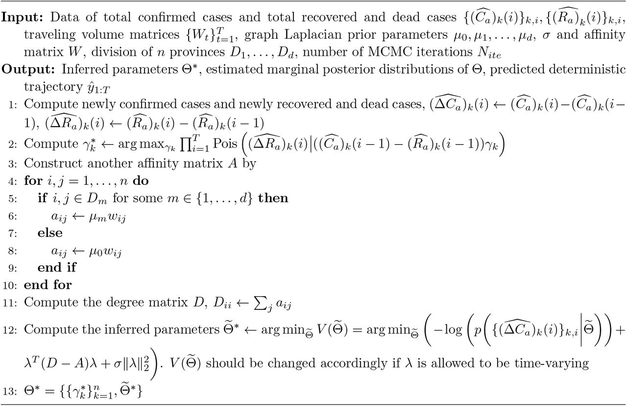
We finally summarize the procedure described in Section 2.2 in Algorithm 1 below.
GLEaM model with Graph Laplacian Prior Distribution


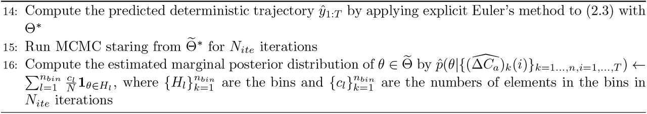
2.3 Prediction of the Epidemic Trajectories with the Estimated Parameters
Once the estimated parameters  are obtained from the optimizations
  and
and  as described in Section 2.2, the trajectories of newly confirmed cases could be simulated according to the stochastic dynamic process with Θ*. Furthermore, trajectories could also be sampled from the posterior distribution of Θ instead of using Θ* alone, which also takes the randomness from
  into account. Particularly, this could be achieved by sampling
  from MCMC and then simulating trajectories with the sampled
  . Additionally, deterministic trajectories determined by (2.3) could also be computed by explicit Euler’s method as in Algorithm 1.
3 Experimental Results for simulated data
Two specific cases are considered for simulated data. The first one considers only two provinces with transportation between each other. In contrast, the other case considers four provinces separated into two groups (the provinces in the same group are assumed to have more similarities) and with traffic between each pair of the provinces.
For each case, we first compare the predicted trajectories of our dynamic model with four baseline models detailed in Section 3.1.2. Comparison between the baseline models shows that heterogeneity of transmission parameters and transportation in the model improves the prediction. Then, the comparison between the baseline models and the proposed model, which further involves the correlation between regions besides heterogeneity and transportation, indicates that the graph Laplacian regularization improves generalization performance. Furthermore, the estimation of transmission parameters using different models shows the benefits of involving heterogeneity of transmission parameters. This also shows that the proposed model can estimate the transmission parameters, validating the capability of the model proposed in this paper in predicting the trajectories. Finally, we show quantitative evaluations of the proposed model and the baseline models by comparing training errors and testing errors defined in Appendix A, which further verifies our findings above.
We remark that the results below are for 100 replicas. In each replica, two random trajectories are sampled according to the stochastic model with prefixed parameters, part of which are treated as the ground truth training and testing trajectory, respectively (see more details in Appendix A). For each model, we first fit the parameters using the training trajectory and then predict the testing trajectory using the estimated parameters. The comparison of trajectory prediction is from one typical realization, for which we compare the ground truth training and testing trajectories with the fitted training and predicted testing trajectories for all the models. Additionally, parameter estimation and quantitative evaluations are compared with mean and standard deviation over all 100 replicas. The detailed computations of training and testing errors for simulated data can be found in Appendix A.
3.1 Two Provinces Case
3.1.1 Data Description
In this case, n = 2. The data span over a period of T = 30 days, and the threshold Tth separating training and testing data is set to be 10 (more detailed can be seen in Appendix A). The other prefixed parameters are as follows:
For k ∈ {1, 2}, Nk(0) = 106, Ek(0) = 30, Hk(0) = 10.
For
.λ1 = 0.4, λ2 = 0.35, δ = γ1 = γ2 = 0.14. {λk} are not time-varying.

3.1.2 Models compared
We first specify the models to be compared below. The last one is the proposed model, and the first four models serve as baselines with different settings.
Models with uniform prior distribution, without heterogeneity or migration.
Models with uniform prior distribution, without heterogeneity but with migration.
Models with uniform prior distribution, with heterogeneity but without migration.
Models with uniform prior distribution, with both heterogeneity and migration.
Models with prior distribution based on graph Laplacian, with both heterogeneity and migration.
First, the models with uniform prior distributions themselves (Models 1-4) are compared according to whether two key assumptions exist in the model:
Whether the transmission rates {λk} are allowed to vary over regions.
Whether there exists transportation between regions.
Then, the model with prior distribution based on graph Laplacian (Model 5) is compared with those using uniform distributions as prior distributions (Models 1-4). The former one utilizes the correlation between subpopulations by adding a l2 regularization term for the model. In contrast, only lower and upper bounds are imposed on parameters without other prior information being used in the latter ones.
Note that for Model 5, that utilizes graph Laplacian based prior distribution as defined in (2.7), the parameter σ is taken to be 10. Moreover, since there are only two provinces in the current experiment, the intra-group parameter {μm, m = 1, 2} does not appear in the final penalty, and only the inter-group parameter determines the graph Laplacian penalty, which is denoted as μ. Specifically, by (2.9),  are estimated by the optimization problem in (3.1):
 We remark that in Models 1-4, the estimation of
  still follows a similar two-step procedure as in Model 5, and the first step of obtaining
  remains formally the same. The difference lies in the optimization object of
  . First, the l2 regularization term becomes prior knowledge of the parameters’ upper and lower bounds. Second, for models without heterogeneity of parameters,
  are forced to be the same in (2.3). For models without transportation between regions, terms involving Wt disappear in (2.3). Additionally, for the other data sets considered in the following sections, the parameter estimation methods for the baseline models are similar and thus will not be repeated.
Finally, note that the model in [11] is similar to Models 1 and 2, since they all assume a spatially homogeneous transmission parameter. However, [11] assumed that the epidemic was seeded from one seed region while Models 1 and 2 do not make such assumption. Moreover, [11] focused more on the spread of the epidemic from the seed region at the early stage of the pandemic, and only the introduction dates in the other regions were utilized for the estimation of transmission parameters. In comparison, the estimation of transmission rate in Models 1 and 2 exploits the data in all regions in the whole process.
3.1.3 Results of Trajectory Comparison
The true trajectories from a typical realization and the predicted trajectories of Models 1-5 are plotted in Figure 1, and the differences of the true trajectories and the fitted trajectories are plotted in Figure 2 for better comparison of the five models.

True and fitted trajectories of Models 1-5 in the two provinces. The vertical lines show the threshold Tth = 10.

Differences of true and fitted trajectories of Models 1-5 in the two provinces. The vertical lines show the threshold Tth = 10.
As can be seen in Figure 1 and 2, Model 4 which allows both heterogeneity and transportation fits the training data better and also predicts the testing data with relatively smaller absolute errors compared with Models 1-3. In addition, Model 5, which further combines the correlation between provinces into prior distribution, has better performance of generalization than Model 4.
3.1.4 Results of Parameter Estimation
The mean and standard deviation of {λi} estimated by the five models are reported in Table 2. It can be seen from Table 2 that models allowing heterogeneity estimate parameters more accurately, and Model 5 that integrates the correlation leads to slightly better estimation for λ2.
Estimated λi of five models. Recall that the ground truth is λ1 = 0.4, λ2 = 0.35. The first three columns indicate whether the model permits migration between provinces, the heterogeneity of parameters and the Graph Laplacian prior, respectively. {λi} are inferred for each of the 100 replicas, then the mean and standard deviation are presented in the table above. In addition, μ = 10−2 in Model 5 for inference of parameters as defined in (3.1).
3.1.5 Further Model Evaluation
The training and testing errors computed according to Appendix A are listed in Table 3 below. From Table 3, it can be seen that even without the prior based on graph Laplacian, heterogeneity of parameters and transportation between two provinces help reduce the testing errors. The concurrence of both the two assumptions makes the training and testing errors further decrease.
Training and testing error with standard deviation for simulated data (two provinces) of five models. The first three columns indicate whether the model permits migration between provinces, the heterogeneity of parameters and the Graph Laplacian prior, respectively. TrainRelErr(1), TestRelErr(1), TrainRelMSE(1) and TestRelMSE(1) are computed for each of the 100 replicas, then the mean and standard deviation are presented in the table above. In addition, μ = 10−2 in Model 5 for inference of parameters as defined in (3.1).
The plots of the mean of TestRelErr(1) and TestRelErr(2) against varying μ are shown in Figure 3. First, note that TestRelErr(1) of Model 4 is nearly the same as that of Model 5 with small μ, since Model 4 is the same as Model 5 with μ = 0. Then, it can be observed from the trend of TestRelErr(1) that as μ decreases, the mean of TestRelErr(1) first decreases and then slightly increases. This indicates that as μ decreases, Model 5 first underfits when μ is large since it forces {λk} to be close to each other, and then overfits when μ is small since nearly no restriction is imposed on {λk}. TestRelErr(1) achieves its minimum when μ is close to 10−2.

Mean of TestRelErr(1) and TestRelErr(2) against μ for simulated data (two provinces). The horizontal green lines show the values of the mean of the testing errors when μ = 0.
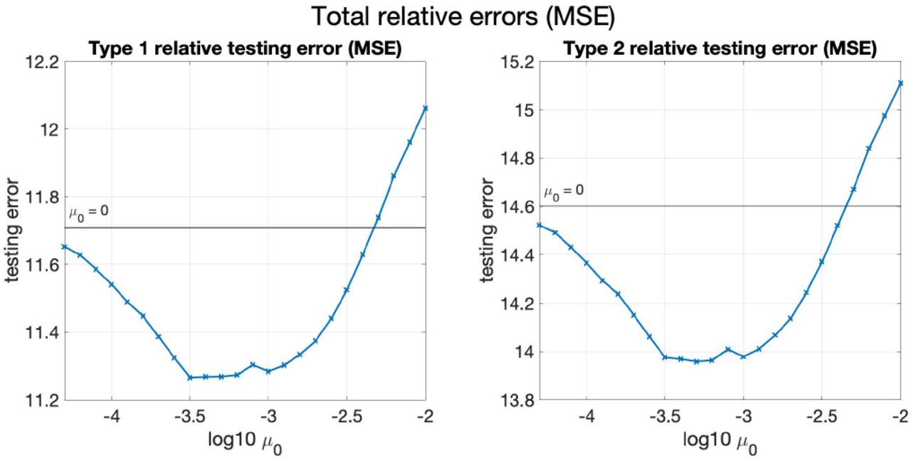
Figure 17 in Appendix C shows relative mean square testing errors against varying μ, in which the same trends described above can be seen.
However, the testing errors are close when μ is relatively small, and thus the benefit of introducing graph Laplacian based prior is less significant in this case. Such a trend is more apparent in the four provinces case in the following subsection.
3.2 Four provinces case
3.2.1 Data Description
In this simulated study, we let n = 4, T = 30, Tth = 10. The other prefixed parameters are listed below:
For k ∈ {1, 2, 3, 4}, Nk(0) = 106, Ek(0) = 30, Hk(0) = 10.
For i ∈ {1, …, T }, k, l ∈ {1, 2, 3, 4} and k ≠ l,
.λ1 = 0.5, λ2 = 0.47, λ3 = 0.4, λ4 = 0.37, δ = γ1 = · · · = γ4 = 0.14. {λk} are not time-varying.
The four provinces are divided into two groups, with the first group consisting of province 1 and 2 and the second group consisting of province 3 and 4. The similarities within groups are reflected in the settings that the values of {λk} are closer for provinces in the same group.
3.2.2 Models compared
The same five models (Models 1-5) as described in Section 3.1.2 are compared for the four provinces case.
Notice that for Model 5, there are three parameters μ0, μ1, μ2 in the graph Laplacian prior, among which μ0 controls the inter-group correlation, μ1 and μ2 control the correlations within group 1 and group 2, respectively. For simplicity of model comparison, we let μ0 = 0 (no restrains on λi’s in different groups), and μ1 = μ2. The parameter σ in (2.7) is still chosen to be 10. Then for Model 5, by (2.9),  are estimated by the optimization problem in (3.2):

3.2.3 Results of Trajectory Comparison
The trajectories of a typical realization are plotted in Figure 4 and the differences between the true and fitted trajectories are shown in Figure 5. As shown in these two figures, heterogeneity helps improve the prediction of testing data more than transportation, while introducing migration without heterogeneity of parameters worsens the estimation as can also be noticed from Table 5. More explanations can be found in Section 3.2.5.
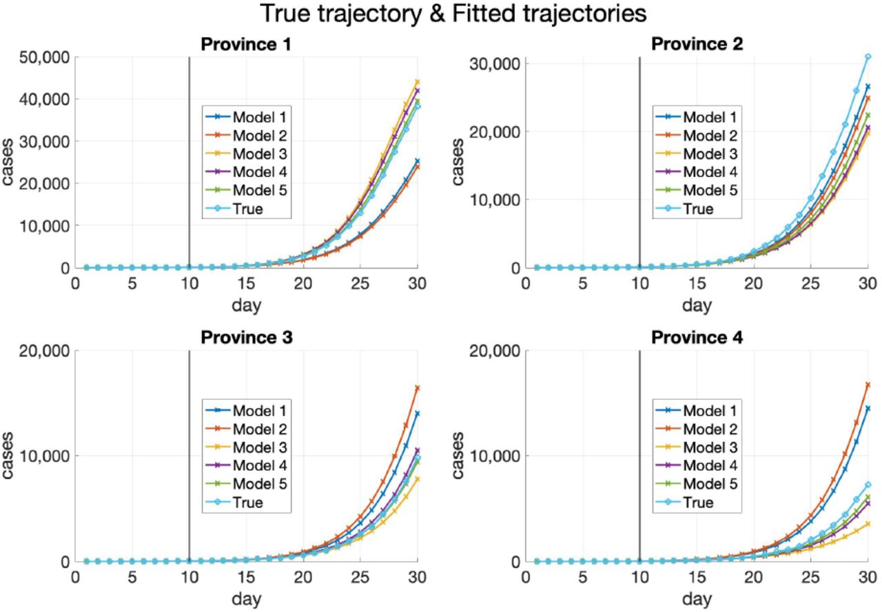
True and fitted trajectories of Models 1-5 in the four provinces. The vertical lines show the threshold Tth = 10.

Differences of true and fitted trajectories of Models 1-5 in the four provinces. The vertical lines show the threshold Tth = 10.
Additionally, Model 5 with prior distrbution based on graph Laplacian lowers the absolute errors of predicted trajectories compared with Model 4.
3.2.4 Results of Parameter Estimation
The mean and standard deviation of {λi} estimated by the five models for four provinces case are reported in Table 4. The same trend as in the two provinces case is observed in the current settings.
Estimated λi of five models. Recall that the ground truth is λ1 = 0.5, λ2 = 0.47, λ3 = 0.4, λ4 = 0.37. The first three columns indicate whether the model permits migration between provinces, the heterogeneity of parameters and the Graph Laplacian prior, respectively. λi are inferred for each of the 100 replicas, and then the mean and standard deviation are presented in the table above. In addition, μ = 10−1.55 in Model 5 for inference of parameters as defined in (3.2).
Training and testing error with standard deviation for simulated data (four provinces) of five models. As in the two provinces case, The first three columns indicate whether the model permits migration between provinces, the heterogeneity of parameters and the Graph Laplacian prior, respectively. TrainRelErr(1), TestRelErr(1), TrainRelMSE(1) and TestRelMSE(1) are still computed for each of the 100 replicas, then the mean and standard deviation are presented in the table above. In addition, μ1 = 10−1.55 in Model 5 for inference of parameters as defined in (3.2).
3.2.5 Further Model Evaluation
The training and testing errors are listed below in Table 5. Different from the two provinces case, it can be seen from Table 5 that the errors increase greatly after transportation is included while heterogeneity remains absent. A possible explanation for this might be that without heterogeneity of parameters and transportation between provinces, the estimated λk’s are lower than the true λk’s for group 1, which leads to that the estimated newly confirmed cases are fewer than the true ones in group 1. For the same reason, the estimated newly confirmed cases are higher than the true ones in group 2. When the transportation is considered, more confirmed cases in group 1 are transferred to group 2 than the cases transported in the opposite direction. As a result, when the transmission parameters do not have heterogeneity, migration between provinces will worsen the prediction performance compared to the case without migration.
In addition, Table 5 still shows that the presence of both heterogeneity and transportation helps reduce the training and testing errors by comparing the first four models. By comparing Model 4 and Model 5, it can be seen that using the graph Laplacian prior could further reduce the testing errors.
As in the previous subsection, the mean of TestRelErr(1) and TestRelErr(2) against varying μ1 is shown below in Figure 6, and the mean of TestRelMSE(1) and TestRelMSE(2) is shown in Figure 18 in Appendix C. From Figure 6 and Figure 18, the phenomenon that Model 5 first underfits and then overfits as μ1 decreases can be seen more recognizably compared with the two provinces case.
Mean of TestRelErr(1) and TestRelErr(2) against μ1 for simulated data (four provinces). The horizontal green lines show the values of the mean of the testing errors when μ1 = 0.
4 Experimental Results for Real-World COVID-19 Data
Real-world COVID-19 data in China and Europe are analyzed in this paper, respectively. Similar to the simulated data cases in Section 3, we first show the predicted trajectories of the proposed model (both deterministic and stochastic ones) and the baseline models (only deterministic ones) for some selected provinces in China or countries in Europe. This shows that the proposed model can capture and further predict the trend of the true trajectories and behaves better than the baseline models, mainly due to the introduction of heterogeneity of transmission parameters and the employment of correlation between provinces or countries. After that, we show the estimation of the posterior distribution of transmission parameters in a selected province or country using the proposed model. Finally, we evaluate the models quantitatively by computing the training and testing errors as described in Appendix A, which further demonstrates the benefits of the proposed model compared to the baselines.
4.1 Data Sources
Real-world data studied in this section involve the data in China and Europe.
Data in China include the number of confirmed cases, recovered cases, and fatalities in China’s major provinces and municipalities from January 21st to March 28th. These publicly available data are downloaded from websites of health commissions of the provinces. The corresponding total population in each province or municipality is from [28].
Transportation data in China are also utilized, lasting from January 10th to February 10th. The data used to reflect the number of people that move out from the cities are collected from Baidu Qianxi [29] (provided by Baidu). This data are collected by keeping track of the locations of smartphones that use the applications from Baidu and can be seen as reflecting the trend of the number of people moving out since Baidu is set as the default search engine for most people in China. Another data set used in this paper reflects the percentage of people moving to the corresponding destinations from their starting points and is also available on [29]. The traveling volume is estimated by combining these two data sets.
Data in Europe include the number of confirmed cases, recovered cases, and fatalities in the following 11 countries from May 1st to August 31st: Denmark, Finland, Norway, Austria, Germany, Switzerland, Italy, Spain, Belgium, France, and Ireland. The data are retrieved from [30, 12]. The corresponding total population in each country is from [31]. However, to our best knowledge, the transportation data between these countries in Europe needed in this model are not publicly available. Thus, the models are simplified when analyzing the European data, and the details can be seen in Section 4.3.
4.2 Results for COVID-19 Data in China
4.2.1 Data Description
After the filtration process described in Appendix B, n = 21 provinces or municipalities are taken into consideration, which are Anhui, Beijing, Fujian, Gansu, Guangdong, Guangxi, Hebei, Henan, Hubei, Hunan, Jiangsu, Jiangxi, Liaoning, Ningxia, Shandong, Shanxi, Shanxi, Shanghai, Sichuan, Zhejiang, and Chongqing.
We set T = 31 (from January 10th to February 10th) and Tth = 27 (February 5st). The data from Tth,1 = 11 (January 21st) to the Tth-th day (February 5st) are treated as the training set, and the data from Tth + 1 (February 6th) to the t-th day (February 10th) are treated as the testing set. In addition, from observation, we choose Tk = 24 (February 2nd) to be the day when λk changes in Anhui, Beijing, Henan and Hubei, and Tk = 20 (January 29th) for the other provinces. More details of the data set can be found in Appendix B.
In addition, the data from Baidu Qianxi might not be the exact traveling volumes between municipalities and provinces. We assume that the actual traveling volume from one starting point to one destination is proportional to the product of numbers of people departed from the stating point and the percentage of population travelling from this origin to the destination. The corresponding scaling parameter α also needs to be inferred from the data for all the models.
4.2.2 Models compared
As in Section 3.1.2, the same Models 1-5 are compared for COVID-19 data in China. Recall that Model 5 is the model proposed in this paper and the other four are the baseline models for comparison.
Note that for Model 5 with prior distribution based on graph Laplacian, the provinces are chosen to be divided into two groups, which are Hubei and other provinces except Hubei, due to the overwhelmed medical resources in Wuhan at the early stage of the pandemic ([32]). For simplicity of comparison, we choose 2μ0 = μ1 = μ2. The parameter σ in (2.7) is chosen to be 1 in this case. Then for Model 5, by (2.9),  and scaling parameter α are estimated by the optimization problem in (4.1):
4.2.3 Results of Trajectory Comparison
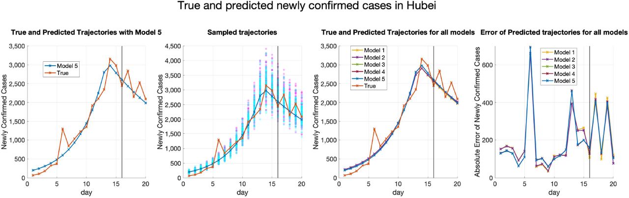
Figure 7 shows the true and predicted trajectories for newly confirmed cases in Hubei. Note that in Figure 7,
The red line shows the true trajectory.
The blue line shows the predicted deterministic trajectories obtained by running (2.3) with Θ* (inferred using (4.1) with μ0 = 10−3.5).
The blue scatter plots show 100 stochastic trajectories with Θ*.
The red scatter plots show 100 stochastic trajectories sampled from the posterior distribution of
(which is estimated by 5 × 10⁵ MCMC iterations staring from ).


True and fitted trajectories in Hubei. The red line shows the true trajectory, the blue line shows the predicted deterministic trajectory with Θ* ( inferred using (4.1) with μ0 = 10−3.5), blue scatter plots show 100 stochastic trajectories with Θ*, and red scatter plots show 100 stochastic trajectories sampled from the posterior distribution of
  (which is estimated by 5 × 10⁵ MCMC iterations staring from
  ). The vertical lines show the threshold Tth = 27 for the training data and testing data.
The deterministic trajectories obtained by the other four models and the corresponding absolute errors are also plotted for better comparison. It can be seen that predicted deterministic trajectories generally capture the trend of the true trajectory. Moreover, sampling trajectories from the posterior distribution of  generates more randomness than sampling trajectories with Θ*. Besides, it can be seen from Figure 7 that the performances of all the five models are similar for Hubei. This may be explained by the fact that the cases in Hubei outnumber those in other provinces or municipalities, which makes all the models tend to fit the trajectory of Hubei best.
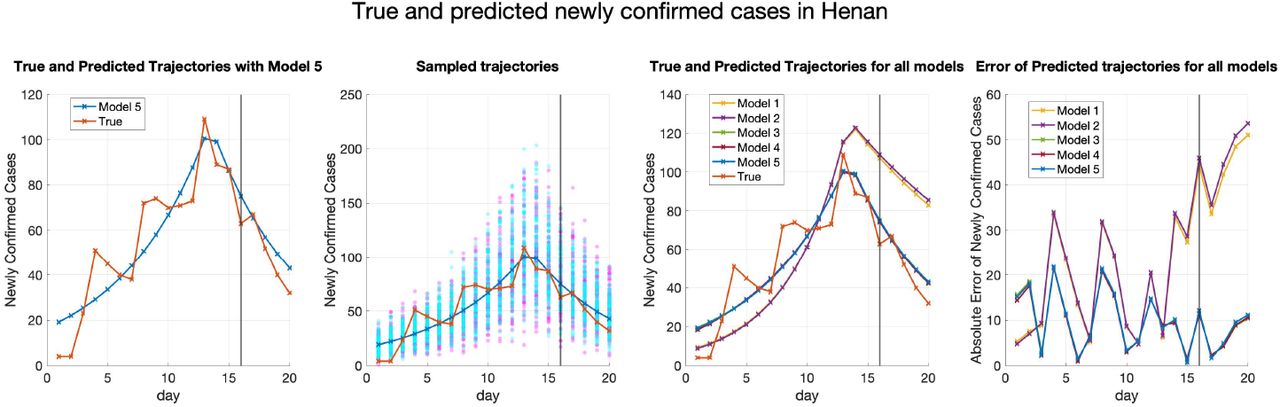
Similarly, Figure 8 shows the predicted trajectories in Henan. As can be seen in Figure 8, unlike Hubei, heterogeneity of parameters helps the model fit and predict the trajectory of Henan in a more significant manner. When the transmission parameters in the two periods are forced to be the same in all provinces, the increment of the newly confirmed cases of the predicted trajectory is faster than the trend shown in the true trajectory in the first period. Meanwhile, the decrement of the newly confirmed cases of the fitted deterministic trajectory in the second period is also slower than the trend reflected in the true trajectory. Thus, heterogeneity helps improve the performance of fitting and predicting.

True and fitted trajectories in Henan. The red line shows the true trajectory, the blue line shows the predicted deterministic trajectory with Θ* ( inferred using (4.1) with μ0 = 10−3.5), blue scatter plots show 100 stochastic trajectories with Θ*, and red scatter plots show 100 stochastic trajectories sampled from the posterior distribution of
  (which is estimated by 5 × 10⁵ MCMC iterations staring from
  ). The vertical lines show the threshold Tth = 27 for the training data and testing data.
Moreover, from Figure 9 which shows the fitted trajectories in Anhui, it can still be seen that heterogeneity helps the models predict the testing trajectory better. Furthermore, introducing correlation helps Model 5 predict the trajectory marginally better than the other models.

True and fitted trajectories in Anhui. The red line shows the true trajectory, the blue line shows the predicted deterministic trajectory with Θ* ( inferred using (4.1) with μ0 = 10−3.5), blue scatter plots show 100 stochastic trajectories with Θ*, and red scatter plots show 100 stochastic trajectories sampled from the posterior distribution of
  (which is estimated by 5 × 10⁵ MCMC iterations staring from
  ). The vertical lines show the threshold Tth = 27 for the training data and testing data.
4.2.4 Results of Parameter Estimation
To illustrate the estimation of the posterior of parameters, Figure 10 shows the estimated posterior distributions of λk,1 and λk,2 in Hubei using Model 5, in which the red lines show the inferred λk,1 and λk,2 with μ1 = 10−3.5, and Table 6 shows the inferred λk,1 and λk,2 with the mean and standard deviation of their estimated posterior distributions from MCMC.
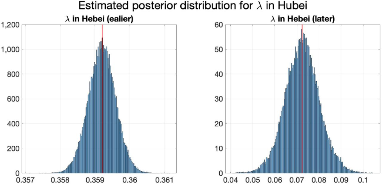
Estimated posterior distribution of λ in Hubei with μ1 = 10−3.5. The vertical red lines represent the values of corresponding θ*.
Estimated paramters in Hubei. θ* is inferred using (4.1) with μ0 = 10−3.5. The posterior distribution is estimated by 5 × 10⁵ MCMC iterations.
By comparing the transmission rates in Hubei in the two periods, it can be seen that the transmission rate decreases greatly after February 2nd, which indicates that the containment measures adopted in Hubei against the COVID-19 outbreak are effective.
4.2.5 Further Model Evaluation
Table 7 shows the training errors and testing errors of the five models computed in the way described in Appendix A. As can be seen from Table 7, both heterogeneity of parameters and transportation between provinces help reduce the training errors and the testing errors as the simulated data case. The utilization of graph Laplacian prior helps further reduce the testing errors. Note that the testing errors of Model 4 are close to those of Model 3, which might be explained as after the traveling restrictions are imposed on January 23rd ([33]), transportation no longer has much influence on the spread of the epidemic.
Training and testing error for real-world data in China of five models. The first three columns indicate whether the model permits migration between provinces, the heterogeneity of parameters and the Graph Laplacian prior, respectively. μ0 = 10−3.5 in Model 5 for inference of parameters as defined in (4.1).
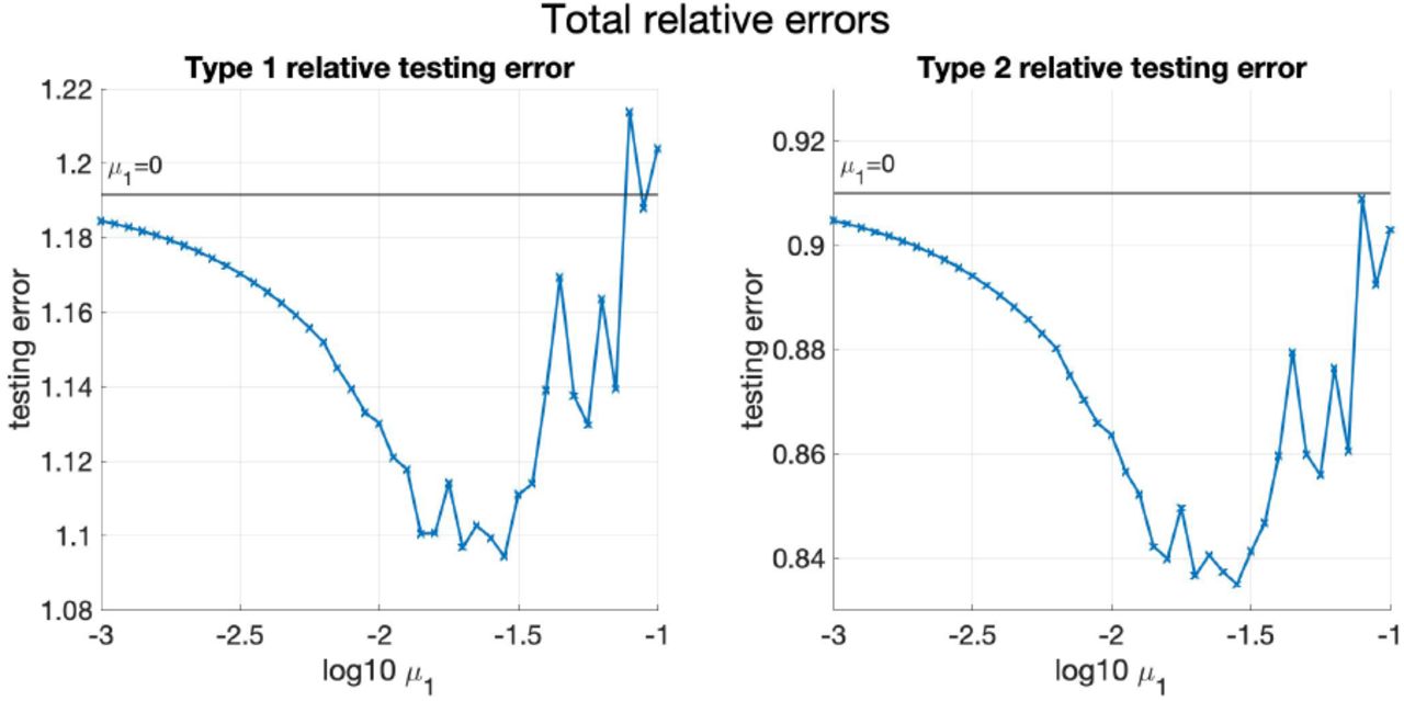
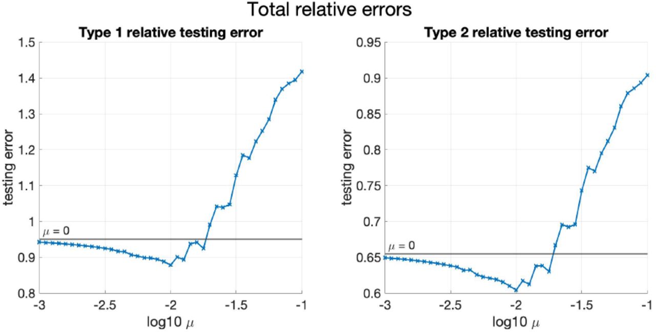
Figure 11 below plots TestRelErr(1) and TestRelErr(2) against varying μ0, and Figure 19 in Appendix C plots TestRelMSE(1) and TestRelMSE(2) against varying μ0. From Figure 11 and Figure 19, it can be observed that Model 5 first underfits and then overfits as μ0 decreases.

TestRelErr(1) and TestRelErr(2) against μ0 for real-world data in China. The horizontal green lines show the values of the mean of the testing errors when μ0 = 0.
4.3 Results for COVID-19 Data in Europe
4.3.1 Data Description
11 countries in Europe are considered in the experiments, which are Denmark, Finland, Norway, Austria, Germany, Switzerland, Italy, Spain, Belgium, France, and Ireland.
Since the original data oscillate much, especially over the weekends, the data are first smoothed by taking a simple moving average (which treats the unweighted average of data in 7 days around the i-th day as the new data point for the i-th day). After the smoothing, T = 116. Additionally, from the observation, Tk = 50 is chosen to be the day when λk changes for all countries except Norway, Italy and France. In addition, TNowway = 75, TItaly = 85 and TFrance = 60. Furthermore, we set Tth = 95.
4.3.2 Models compared
For COVID-19 data in Europe, only three models detailed below are compared, which allow heterogeneity of parameters but do not include transportation. The transportation data needed in this model are not available to the best of our knowledge. However, the impact of transportation is expected to be less significant due to travel restrictions [33].
1’. Model with uniform prior distribution, without heterogeneity or migration.
2’. Model with uniform prior distribution, with heterogeneity but without migration.
3’. Model with prior distribution based on graph Laplacian, with heterogeneity but no migration.
For Model 3’, 11 countries are partitioned into d = 4 groups:
Northern Europe: Denmark, Finland, Norway;
Central Europe: Austria, Germany, Switzerland;
Southern Europe: Italy, Spain;
Western Europe: Belgium, France, Ireland,
Besides, in Model 3’, we assume that μ1 = · · · = μd = μwithin, μ0 = μbetween, and μwithin = 10μbetween for simplicity. The parameter σ in the prior distribution (2.7) is still taken to be 1. Then by (2.9), for Model 3’,  are estimated by the optimization problem in (4.2):
 where w = 105 is a constant scaling.
4.3.3 Results of Trajectory Comparison
Figure 12, 13 and 14 present the true and predicted trajectories in Austria, Germany, and Italy, respectively. As can be seen from Figure 12, 13 and 14, heterogeneity of transmission parameters in Model 2’ and Model 3’ helps improve the performance of fitting and generalization. Furthermore, utilization of correlation between countries in Model 3’ further improves the prediction of the trajectories.

True and fitted trajectories in Austria. The red line shows the true trajectory, the blue line shows the predicted deterministic trajectory with Θ* ( inferred using (4.2) with μbetween = 10−1), blue scatter plots show 100 stochastic trajectories with Θ*, and red scatter plots show 100 stochastic trajectories sampled from the posterior distribution of
  (which is estimated by 5 × 10⁵ MCMC iterations staring from
  ). The vertical lines show the threshold Tth = 95 for the training data and testing data.

True and fitted trajectories in Germany. The red line shows the true trajectory, the blue line shows the predicted deterministic trajectory with Θ* ( inferred using (4.2) with μbetween = 10−1), blue scatter plots show 100 stochastic trajectories with Θ*, and red scatter plots show 100 stochastic trajectories sampled from the posterior distribution of
  (which is estimated by 5 × 10⁵ MCMC iterations staring from
  ). The vertical lines show the threshold Tth = 95 for the training data and testing data.
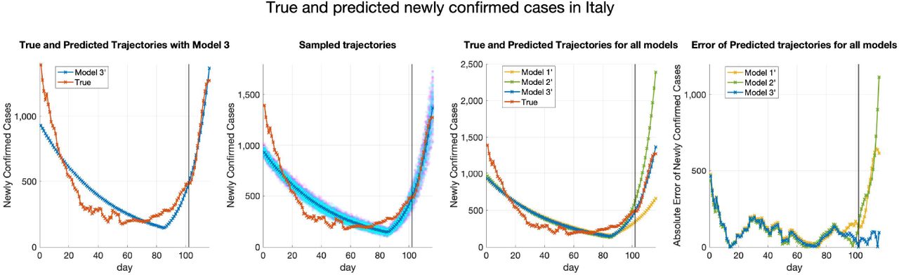
True and fitted trajectories in Italy. The red line shows the true trajectory, the blue line shows the predicted deterministic trajectory with Θ* ( inferred using (4.2) with μbetween = 10−1), blue scatter plots show 100 stochastic trajectories with Θ*, and red scatter plots show 100 stochastic trajectories sampled from the posterior distribution of
  (which is estimated by 5 × 10⁵ MCMC iterations staring from
  ). The vertical lines show the threshold Tth = 95 for the training data and testing data.
4.3.4 Results of Parameter Estimation
Same as before, Figure 15 shows the estimated posterior distributions of λk,1 and λk,2 in Italy using Model 3’, in which the red lines show the inferred λk,1 and λk,2 with μbetween = 1. Table 8 shows the inferred λk,1 and λk,2 and the mean and standard deviation of their estimated posterior distribution from MCMC.
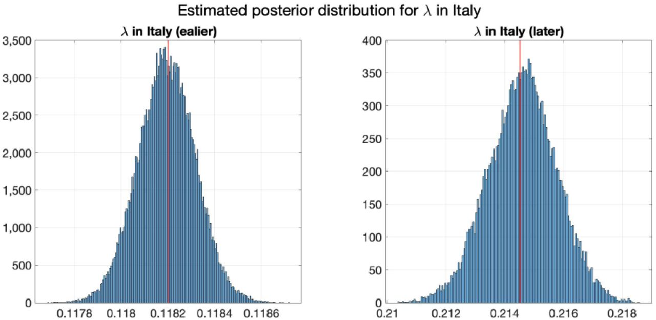
Estimated posterior distributions of λ in Italy with μbetween = 10−1. The vertical red lines represent the values of corresponding θ*.
Estimated paramters in Italy. θ* is inferred using (4.2) with μbetween = 10−1. The posterior distribution is estimated by 5 × 10⁵ MCMC iterations.
4.3.5 Further Model Evaluation
Table 9 shows training and testing errors of the three models. It can be seen from Table 9 that heterogeneity of transmission parameters helps reduce both training and testing errors. We can also see that adding Graph Laplacian prior properly further reduces the testing errors greatly without increasing training errors much.
Training and testing error for real-world data in Europe of five models. The first three columns indicate whether the model permits migration between provinces, the heterogeneity of parameters and the Graph Laplacian prior, respectively. μ0 = 10−1 in Model 3’ for inference of parameters as defined in (4.1).
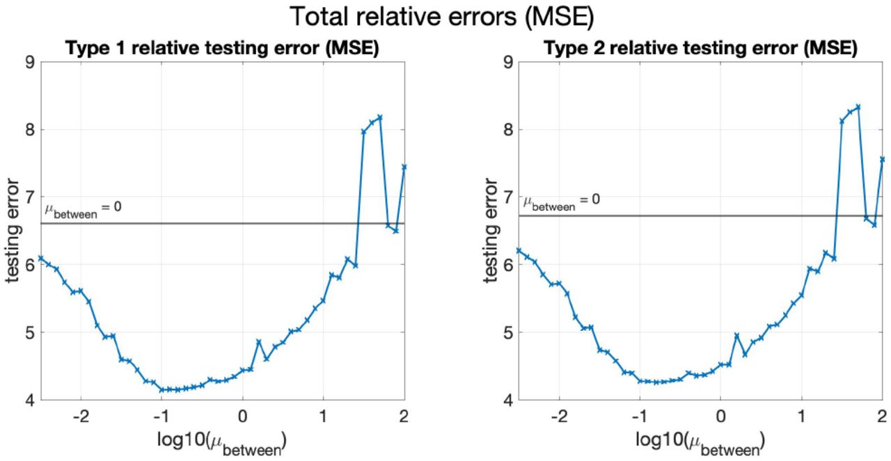
Figure 16 below and Figure 20 in Appendix C plot TestRelErr(1), TestRelErr(2), TestRelMSE(1) and TestRelMSE(2) against varying μbetween, from which one may see the same trend of prediction performance as μbetween varies.

TestRelErr(1) and TestRelErr(2) against μbetween for real-world data in Europe. The horizontal green lines show the values of the mean of the testing errors when μbetween = 0.

Mean of TestRelMSE(1) and TestRelMSE(2) against μ for simulated data (two provinces). The horizontal green lines show the values of the mean of the testing errors when μ = 0.

Mean of TestRelMSE(1) and TestRelMSE(2) against μ1 for simulated data (four provinces). The horizontal green lines show the values of the mean of the testing errors when μ1 = 0.
5 Discussion
In this paper, we propose a stochastic dynamic model inspired by [1], considering the inter-district transportation and both spatially and temporally heterogeneous transmission parameters, which can model the ongoing and lasting spread of the epidemic in multiple districts. Based on this model, we also introduce a two-step procedure for estimating the parameters, which maximizes over posterior distribution with a prior distribution that utilizes graph Laplacian regularization to address the correlation between districts. Experiments on both simulated and real-world data show that compared with the baseline models, this new model with transportation, heterogeneity of parameters, and usage of the correlation in parameter inference improves the performance of fitting and generalization.
We acknowledge that there are limitations in this work. First, the stochastic dynamic model proposed in this paper might not be comprehensive enough to characterize the spread of COVID-19 in reality. For example, the model does not account for the asymptomatic virus carriers and the infectious incubation period. Second, the proposed model does not consider the heterogeneity of risk of being infected in different populations, for example, populations with different ages, jobs, or health conditions. Third, The proposed model needs further modification considering the large-scale COVID-19 vaccination. At last, the current method does not provide the guidance to determine how intensively we would like to stress the correlation between districts.
The current methods have possible extensions in the following several directions in the future study. First, the dynamic model is to be refined to be closer to reality, for example, taking the asymptomatic virus carriers and medical tracking into account and allowing the change of the transmission parameters as time increases to be more realistic. Second, the model can be modified to accommodate the heterogeneity of various populations, including different age groups and vaccination statuses. For example, the compartments S, E, H, R are to be further divided into subgroups, and the parameters such as transmission rates and mortality rates are allowed to be different; meanwhile, the dynamic model is also to be adjusted accordingly. At last, the method could be further used to assess the influence of containing measures taken by different countries, for example, through adjusting the traveling volume to make it different from the actual transportation data and then analyzing the corresponding changes in newly confirmed cases.
Data Availability
All data produced in the present study are available upon reasonable request to the authors
Acknowledgement
The authors thank Dr. Huaiyu Tian for helpful discussion. Yuan Zhang and Xiao-Hua Zhou are funded by National Natural Science Foundation of China grant 8204100362 and The Bill & Melinda Gates Foundation (INV-016826). Yixuan Tan and Xiuyuan Cheng are funded by NSF (DMS-2007040) and the Alfred P. Sloan Foundation.
Appendix A Model Evaluation Metric
Measurements are proposed in this section to evaluate the performance of fitting and generalization of the aforementioned models in the experiments section.
To be more specific, the performance of fitting is measured on the training data  up to some threshold Tth, and the performance of generalization is evaluated on the testing data
  . Note that Tth should not be earlier than the maximum of Tk, which is the day that λk changes in the k-th region, ∀k = 1, …, n.
For both simulated and real-world data, the fitting performance is assessed by comparing the training data  with the fitted deterministic trajectory
  , which is obtained by integrating ODE system (2.3) whose parameters
  are inferred by the corresponding model.
Similarly, the generalization performance is assessed by comparing the testing data  with the predicted deterministic trajectory
  obtained by integrating (2.3) with parameters Θ. Although the deterministic trajectory is still computed by ODE system (2.3), its initialization is the number of individuals in compartments on the Tth-th day of the testing data, i.e., {Sk(Tth), Ek(Tth), Hk(Tth), Rk(Tth), k = 1, …, n}. Then, the trajectory
  is obtained by running (2.3) for T − Tth days with the transmission parameters
  .
.
Simulated data
For simulated data, two random trajectories are sampled according to the stochastic model with prefixed parameters in one replica. Data from the first Tth days of one trajectory are treated as the training data, and data from the last T − Tth days of the other trajectory are treated as the testing data. This guarantees that the training and testing data are independent.
Besides, the prestored {Sk(Tth), Ek(Tth), Hk(Tth), Rk(Tth)} of the testing trajectory are used as the initialization of (2.3) to obtain the deterministic trajectory  as described above.
real-world data
For real-world data, only one observable trajectory is available, thus the training data and the testing data are the two parts of the true trajectory split by the Tth-th day.
In contrast to the case for simulated data, for real-world data, only  are available, while {Ek(Tth), Hk(Tth), Rk(Tth)} are not known. Therefore, trajectories starting from the Tth +1-th day can not be computed directly. Instead, a deterministic trajectory for all the T days is computed with the fitted parameters Θ, and then the data for the first Tth days and for the last T − Tth days are treated as
  and
and  , respectively.
Based on the explanations above, the training errors and testing errors can be defined. Details are listed below.
Remind that the ground truth training data and testing data are  and
and  , respectively. In addition, the fitted deterministic training trajectories and predicted deterministic testing trajectories with parameters Θ are denoted as
  and
and  , respectively. The details of obtaining training data, testing data along with fitted trajectories for both simulated data and real-world data have been explained above.
Based on the ground truth trajectories and the fitted ones, define

 which denote the absolute error and relative error for the training data in the k-th region on the i-th day, respectively.
With the errors defined for each day, the total errors for the k-th region are the weighted sums of  and
and  . There exist two types of reasonable weights for weighting the errors. The first type is defined as
 which share with same trend of increasing or decreasing as the newly confirmed cases in the k-th region.
Moreover, the second type of weights is the simple average of errors for all the T days, that is to say,
 With the weights defined as (A.3) or (A.4), the total absolute or relative training errors or mean square errors for the k-th region can be correspondingly defined as


 where j ∈ {1, 2}. After defining the errors for each region, the total errors are defined as the summation of the errors of all the regions,


 In addition, the testing errors and weights are defined in the same way as above, which are listed below,
Absolute error and relative error of the k-th region on the i-th day:
Two kinds of weights:
Weighted absolute error and relative error of the k-th region:
Weighted absolute and relative mean square error of the k-th region:
Total weighted absolute and relative error:
Total weighted absolute and relative mean square error:


In the above definitions, i ∈ {1, …, T }, k ∈ {1, …, n}, j ∈ {1, 2}.
Appendix B Preprocessing of real-world data in China
Filtration of Provinces in China
For stability of inference for parameters, only the provinces or municipalities whose accumulated confirmed cases are above 50, the estimated δk are not less than 10−10 and the change of λk occurs no later than February 2nd are considered.
Description of real-world data in China
The COVID-19 data including the number of confirmed cases, recovered cases and fatalities in major provinces and cities of China are from January 21st to March 28th. Moreover, the transportation data are from January 10th to February 10th. Thus, we consider the spread of COVID-19 in China from January 10th to February 10th, and T = 31. However, only the COVID-19 after January 21st are available, hence the training set is the data from Tth,1 = 11 (January 21st) to the Tth-th day (February 5st), and the testing set is the data from Tth + 1 (February 6th) to the t-th day (February 10th).
Appendix C Supplementary Figures

TestRelMSE(1) and TestRelMSE(2) against μ0 for real-world data in China. The horizontal green lines show the values of the mean of the testing errors when μ0 = 0.
TestRelMSE(1) and TestRelMSE(2) against μbetween for real-world data in Europe. The horizontal green lines show the values of the mean of the testing errors when μbetween = 0.
References


