
Abstract
Phylodynamic methods reveal the spatial and temporal dynamics of viral geographic spread, and have featured prominently in studies of the COVID-19 pandemic. Virtually all previous studies are based on phylodynamic models that assume—despite direct and compelling evidence to the contrary—that rates of viral geographic dispersal are constant through time. Here, we: (1) extend phylodynamic models to allow both the average and relative rates of viral dispersal to vary independently between pre-specified time intervals; (2) implement methods to infer the number and timing of viral dispersal events between areas; and (3) develop statistics to assess the absolute fit of phylodynamic models to empirical datasets. We first validate our new methods using analyses of simulated data, and then apply them to a SARS-CoV-2 dataset from the early phase of the COVID-19 pandemic. We show that: (1) under simulation, failure to accommodate interval-specific variation in the study data will severely bias parameter estimates; (2) in practice, our interval-specific phylodynamic models can significantly improve the relative and absolute fit to empirical data; and (3) the increased realism of our interval-specific phylodynamic models provides qualitatively different inferences regarding key aspects of the COVID-19 pandemic—revealing significant temporal variation in global viral dispersal rates, viral dispersal routes, and number of viral dispersal events between areas—and alters interpretations regarding the efficacy of intervention measures to mitigate the pandemic.
Phylodynamic methods are increasingly used to understand the spatial and temporal spread of disease outbreaks and have been used extensively to infer key aspects of the COVID-19 pandemic, such as the geographic location and time of origin of the disease, the rates and geographic routes by which it spread, and the efficacy of various mitigation measures to limit its geographic expansion (1–15). Phylodynamic methods adopt an explicitly probabilistic approach that models the process of viral dispersal among a set of discrete geographic areas (16). The observations include the times and locations of viral sampling, and the genomic sequences of the sampled viruses. These data are used to estimate the parameters of phylodynamic models, which include a dated phylogeny of the viral samples, the global dispersal rate (the average rate of dispersal among all geographic areas), and the relative dispersal rates (the dispersal rate between each pair of geographic areas).
The vast majority (651 of 666, 97.7%; Fig. S1) of phylodynamic studies are based on the earliest models (17, 18), which assume that viral dispersal dynamics—including the average and relative rates of viral dispersal— remain constant over time. However, real-world observations indicate that the average and/or relative rates of viral dispersal inevitably vary during disease outbreaks. For example, relative rates of viral dispersal typically change as a disease is introduced to (and becomes prevalent in) new areas, and begins dispersing from those areas to other areas. Dispersal dynamics are also generally impacted by the initiation (or alteration or cessation) of area-specific mitigation measures (e.g., domestic shelter-in-place policies) that change the rate of viral transmission within an area and the relative rate of dispersal to other areas. Similarly, average rates of viral dispersal may change in response to the initiation (or alteration or cessation) of more widespread intervention efforts—e.g., multiple areaspecific mitigation measures, international-travel bans—that collectively impact the overall viral dispersal rate.
In this paper, we: (1) extend phylodynamic models to allow both the average and relative dispersal rates to vary independently between pre-specified time intervals; (2) enable stochastic mapping under these interval-specific phylodynamic models to estimate the number and timing of viral dispersal events between areas, and; (3) develop statistics to assess the absolute fit of phylodynamic models to empirical datasets. We first validate the theory and implementation of our new phylodynamic methods using analyses of simulated data, and then provide an empirical demonstration of these methods with analyses of a SARS-CoV-2 dataset from the early phase of the COVID-19 pandemic. We show that: (1) under simulation, failure to accommodate interval-specific variation in the dispersal process can bias epidemiological estimates; (2) in practice, our interval-specific phylodynamic models have the potential to significantly improve the relative and absolute fit to empirical data, and; (3) the increased realism of our interval-specific phylodynamic model provides qualitatively different inferences regarding key aspects of the COVID-19 pandemic—revealing significant temporal variation in global viral dispersal rates, viral dispersal routes, and number of viral dispersal events between areas—and alters interpretations regarding the efficacy of mitigation measures to limit the pandemic.
Accommodating Variation in Viral Dispersal Dynamics
Anatomy of interval-specific phylodynamic models
Phylodynamic models include two main components (Fig. 1): a phylogenetic model that allows us to estimate a dated phylogeny for the sampled viruses, Ψ, and a biogeographic model that describes the history of viral dispersal over the tree as a continuous-time Markov chain. For a geographic history with k discrete areas, this stochastic process is fully specified by a k ×k instantaneous-rate matrix, Q, where an element of the matrix, qij, is the instantaneous rate of change between state i and state j (i.e., the instantaneous rate of dispersal from area i to area j). We rescale the Q matrix such that the average rate of dispersal between all areas is μ; this represents the average rate of viral dispersal among all areas.

Phylodynamic models include two main components: a phylogenetic model that specifies the relationships and divergence times of the sampled viruses, Ψ (top panel), and a biogeographic model that describes the history of viral dispersal among a set of discrete geographic areas—here, areas 1 (orange), 2 (blue), and 3 (green)—from the root to the tips of the dated viral tree. Parameters of the biogeographic model include an instantaneous-rate matrix, Q, that specifies relative rates of viral dispersal between each pair of areas (here, each element of the matrix, qij, is represented as an arrow that indicates the direction and relative dispersal rate from area i to area j; middle panel), and a parameter that specifies the average rate of viral dispersal between all areas, μ (lower panel). Although most phylodynamic studies assume that the process of viral dispersal is constant through time, disease outbreaks are typically punctuated by events that impact the average and/or relative rates of viral dispersal among areas. Here, for example, the history involves two events (e.g., mitigation measures) that define three intervals, where both Q and μ are impacted by each of these events, such that the interval-specific parameters are (Q1,Q2,Q3) and (μ1,μ2,μ3). Our framework allows investigators to specify phylodynamic models with two or more intervals, where each interval has independent relative and/or average dispersal rates, which are then estimated from the data.
We could specify alternative biogeographic models based on the assumed constancy of the dispersal process. For example, the simplest possible model assumes that the average dispersal rate, μ, and the relative dispersal rates, Q, remain constant over the entire history of the viral outbreak. Typically, viral outbreaks are punctuated by events that are likely to impact the average rate of viral dispersal (e.g., the onset of an international-travel ban) and/or the relative rates of viral dispersal between pairs of areas (e.g., the initiation of localized mitigation measures). We can incorporate information on such events into our phylodynamic inference by specifying interval-specific models. That is, the investigator specifies the number of intervals, the boundaries between each interval, and the parameters that are specific to each interval according to the presumed changes in the history of viral dispersal. For example, we might specify an interval-specific model (19) that assumes that the average rate of viral dispersal varies among two or more intervals (while assuming that the relative rates of viral dispersal remain constant across intervals). Conversely, an interval-specific model (20) might allow the relative rates of viral dispersal to vary among two or more time intervals (while assuming that the average rate of viral dispersal remains constant across intervals). Alternatively, a more complex interval-specific model might allow both the average rate of viral dispersal and the relative rates of viral dispersal to vary among two or more intervals. By accommodating potential variation in both average and relative rates of viral dispersal, and by allowing us to incorporate additional information regarding events that may impact viral dispersal, interval-specific models may improve the realism of phylodynamic models, thereby increasing the accuracy of our epidemiological inferences based on these models.
Inference under interval-specific phylodynamic models
We estimate parameters of the interval-specific phylodynamic models within a Bayesian statistical framework. Specifically, we use numerical algorithms—Markov chain Monte Carlo simulation—to approximate the joint posterior probability distribution of the phylodynamic model parameters—the dated phylogeny, Ψ, the set of relative dispersal rates, Q, and the average dispersal rates, μ—from the study data (i.e., the location and times of viral sampling, and the genomic sequences of the sampled viruses).
We have also implemented numerical algorithms—stochastic mapping—to simulate histories of viral dispersal under interval-specific phylodynamic models; these methods allow us to estimate the number of dispersal events between a specific pair of areas, the number of dispersal events from one area to a set of two or more areas, or the total number dispersal events among all areas. We also leverage our ability to simulate histories under interval-specific phylodynamic models to develop new methods to assess the absolute fit of phylodynamic models to empirical datasets (described below).
Assessing the relative and absolute fit of interval-specific phylodynamic models
For a given phylodynamic study, we might wish to consider several candidate interval-specific models (where each candidate model specifies a unique interval number, interval boundaries, and/or interval-specific parameters). Comparing the fit of these competing phylodynamic models to our study data offers two important benefits: (1) confirming that our inference model provides an adequate description of the process that gave rise to our study data will ensure the accuracy of the corresponding inferences (i.e., our estimates of relative and/or average dispersal rate parameters and viral dispersal histories), and; (2) comparing alternative models provides a means to objectively test hypotheses regarding the impact of events on the history of viral dispersal (i.e., by assessing the relative fit of our data to competing models that are specified to include/exclude the impact of a putative event on the average and/or relative viral dispersal rates).
We assess the relative fit of two or more candidate phylodynamic models to a given dataset using Bayes factors; this requires that we first estimate the marginal likelihood for each model (which represents the average fit of a model to a dataset), and then compute the Bayes factor as twice the difference in the log marginal likelihoods of the competing models (21).
We assess the absolute fit of a candidate phylodynamic model using posterior-predictive assessment (22). This Bayesian approach for assessing model adequacy is based on the following premise: if our inference model provides an adequate description of the process that gave rise to our observed data, then we should be able to use that model to simulate datasets that resemble our original data. The resemblance between the observed and simulated datasets is quantified using a summary statistic. We developed two summary statistics to assess the adequacy of interval-specific phylodynamic models: (1) the parsimony statistic (calculated as the difference in the minimum number of dispersal events required to explain the observed data versus the number required for a simulated dataset), and; (2) the tipwise-multinomial statistic (calculated as the difference in the multinomial probabilities for observed set of areas at the tips of the tree versus the set of simulated areas). We provide detailed descriptions of the statistical model, inference machinery, model-comparison methods, and implementation in Section 1 of the SI Appendix.
Simulation Study
We performed a simulation study to explore the statistical behavior of the interval-specific phylodynamic models. Specifically, the goals of this simulation study are to assess: (1) our ability to perform reliable inference under interval-specific models; (2) the impact of model misspecification, and; (3) our ability to identify the correct model. To this end, we simulated 200 geographic datasets under each of two models: the first assumes a constant μ and Q (1μ1Q), and the second allows μ and Q to vary over two intervals (2μ2Q). For each simulated dataset, we separately inferred the history of viral dispersal under each model, resulting in four true:inference model combinations: 1μ1Q:1μ1Q, 2μ2Q:2μ2Q, 1μ1Q:2μ2Q, and 2μ2Q:1μ1Q. We provide detailed descriptions of the simulation analyses and results in Section 2 of the SI Appendix.
Ability to reliably estimate parameters of interval-specific phylodynamic models
Interval-specific phylodynamic models are inherently more complex than their constant counterparts, and therefore contain many more parameters that must be inferred from geographic datasets that contain minimal information; these datasets only include a single observation (i.e., the area in which each virus was sampled). These considerations raise concerns about our ability to reliably estimate parameters of interval-specific phylodynamic models. Encouragingly, when the inference model is correctly specified (i.e., where both the true and inference models include [or exclude] interval-specific parameters, 2μ2Q:2μ2Q and 1μ1Q:1μ1Q), our simulation study demonstrates that estimates under interval-specific models are as reliable as those under constant models (Fig. 2, green, blue). Moreover, when the inference model is overspecified (i.e., it includes interval-specific parameters not included in the true model) inferences are comparable to those under correctly specified models (Fig. 2, purple). However, when the inference model is underspecified (i.e., it excludes interval-specific parameters of the true model) inferences are severely biased estimates (Fig. 2, orange).

We simulated 200 geographic datasets under each of two models: one that assumed a constant μ and Q (1μ1Q), and one that allowed μ and Q to vary over two intervals (2μ2Q). For each simulated dataset, we separately inferred the total number of dispersal events under each model, resulting in four true:inference model combinations (1μ1Q:1μ1Q, 2μ2Q:2μ2Q, 1μ1Q:2μ2Q, and 2μ2Q:1μ1Q). Left) For each combination of true and inference model, we computed the coverage probability (the frequency with which the true number of dispersal events was contained in the corresponding X% credible interval; y-axis) as a function of the size of the credible interval (x-axis). When the model is true, we expect the coverage probability to be equal to the size of the credible interval (23). As expected, coverage probabilities fall along the one-to-one line when the model is correctly specified (green and blue). Moreover, coverage probabilities are also appropriate when the inference model is overspecified (i.e., the inference model includes interval-specific parameters not included in the true model; purple). However, coverage probabilities are extremely unreliable when the inference model is underspecified (i.e., the inference model excludes interval-specific parameters of the true model; orange). Right) For each true:inference model combination, we summarized the absolute error (estimated minus true number of dispersal events) as boxplots (median [horizontal bar], 50% probability interval [boxes], and 95% probability interval [whiskers]). Again, when the model is underspecified (orange) inferences are strongly biased compared to those under the correctly specified (green and blue) and overspecified (purple) models.
Ability to accurately identify an appropriately specified phylodynamic model
Our simulation study demonstrates the importance of identifying scenarios where an inference model is underspecified; failure to accommodate interval-specific variation in the study data will severely bias parameter estimates. Fortunately, our simulation study demonstrates that we can reliably identify when a given model is correctly specified, overspecified, or underspecified using a combination of Bayes factors (to assess the relative fit of competing models to the data; Fig. 3, left) and posterior-predictive simulation (to assess the absolute fit of each candidate model to the data; Fig. 3, right). Using a combination of Bayes factors and posterior-predictive simulation allows us to not only identify the best of the candidate models, but also to ensure that the best model provides an adequate description of the true process that gave rise to our study data.

We assessed the relative and absolute fit of alternative models to the simulated datasets described in Fig. 2. Left) For each simulated dataset, we compared the relative fit of the true and alternative models using Bayes factors. The boxplots summarize Bayes factors for datasets simulated under the constant (1μ1Q, left) and interval-specific (2μ2Q, right) models, which demonstrate that we are able to decisively identify the true phylodynamic model. Right) For each combination of true:inference model, we assessed absolute model fit using posterior-predictive simulation with a set of 20 summary statistics. Each dot represents the fraction of those 20 summary statistics for which the corresponding inference model provides an inadequate fit to a single simulated dataset. The violin plots summarize the distribution of these values for all datasets under each true:inference model combination. As expected, the true model is overwhelmingly inferred to be adequate (green and blue). Encouragingly, model overspecification appears to have a negligible impact on model adequacy (purple). By contrast, an underspecified model severely impacts model adequacy (orange).
Empirical Application
We illustrate our new phylodynamic methods with analyses of all publicly available SARS-CoV-2 genomes sampled during the early phase of the COVID-19 pandemic (with 2598 viral genomes collected from 23 geographic areas between Dec. 24, 2019–Mar. 8, 2020). We used our study dataset to estimate the parameters of—and assess the relative and absolute fit to—nine candidate phylodynamic models. These models assign interval-specific parameters—for the average rate of viral dispersal, μ, and/or relative rates of viral dispersal, Q—to one, two, four, or five pre-specified time intervals; i.e., 1μ1Q, 2μ1Q, 1μ2Q, 2μ2Q, 4μ1Q, 1μ4Q, 4μ4Q, 5μ5Q, and 5μ5Q*. We specified interval boundaries based on external information regarding events within the study period that might plausibly impact viral dispersal dynamics, including: (A) start of the Spring Festival travel season in China (the highest annual period of domestic travel, Jan. 12); (B) onset of mitigation measures in Hubei province, China (Jan. 26); (C) onset of international air-travel restrictions against China (Feb. 2), and; (D) relaxation of domestic travel restrictions in China (Feb. 16). Phylodynamic models with two intervals include event C, models with four intervals include events A, C, and D, and the 5μ5Q model includes all four events. The final candidate model, 5μ5Q*, includes five arbitrary and uniform (bi-weekly) intervals. We provide detailed descriptions of our empirical data collection, analyses, and results in Section 3 of the SI Appendix.
An interval-specific model best describes viral dispersal in the early phase of the pandemic
Our phylodynamic analyses of the SARS-CoV-2 dataset reveal that the early phase of the COVID-19 pandemic exhibits significant variation in both the average and relative rates of viral dispersal over four time intervals. Bayes factor comparisons (Fig. 4, left) demonstrate that the 4μ4Q interval-specific phylodynamic model is decisively preferred both over all less complex candidate models—including models that allow either the average dispersal rate or relative dispersal rates to vary over the same four intervals (4μ1Q and 1μ4Q, respectively)—and also over more complex candidate models (5μ5Q, and 5μ5Q*). Posterior-predictive analyses (Fig. 4, right) demonstrate that the preferred model, 4μ4Q, also provides an adequate description of the process that gave rise to our SARS-CoV-2 dataset. Below, we will use the preferred (4μ4Q) interval-specific phylodynamic model to explore various aspects of viral dispersal during the early phase of the COVID-19 pandemic and—for the purposes of comparison—we also present corresponding results inferred using the (underspecified) constant (1μ1Q) phylodynamic model.
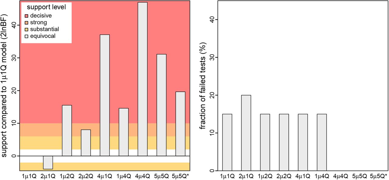
We assessed the relative and absolute fit of nine candidate phylodynamic models to our study dataset (comprised of all publicly available SARS-CoV-2 genomes from the early phase of the COVID-19 pandemic). Left) We compared the relative fit of each candidate model to the constant (1μ1Q) phylodynamic model using Bayes factors, which indicate that the 4μ4Q interval-specific model outcompetes both less complex and more complex models. Right) We performed posterior-predictive simulation for each candidate model using 20 summary statistics, plotting the fraction of those summary statistics indicating that a given candidate model was inadequate. Our results indicate that three candidate models (4μ4Q, 5μ5Q, and 5μ5Q*) provide an adequate fit to our SARS-CoV-2 dataset. The simplest of these adequate models (4μ4Q) also provides the best relative fit. Collectively, these results identify the 4μ4Q model as the clear choice for phylodynamic analyses of our study dataset.
Variation in global viral dispersal rates
Between late 2019 and early March, 2020, COVID-19 emerged (in Wuhan, China) and established a global distribution—with reported cases in 83% of the study areas by this date (24)—despite the implementation of numerous intervention efforts to slow the spread of the causative SARS-CoV-2 virus (25). This crucial early phase of the pandemic provides a unique opportunity to explore the dispersal dynamics that led to the worldwide establishment of the virus and to assess the efficacy of key public-health measures to mitigate the spread of COVID-19. The constant (1μ1Q) model infers a static rate of global viral dispersal throughout the study period (Fig. 5, orange). By contrast, inferences under the preferred (4μ4Q) model reveal significant variation in global viral dispersal rates over four intervals, exhibiting both increases and decreases over the early phase of the pandemic (Fig. 5, dark blue). The significant decrease in the global viral dispersal rate between the second and third interval (with a boundary at Feb. 2) coincides with the initiation of international air-travel bans with China (imposed by 34 countries and nation states by this date). To further explore the possible impact of the air-travel ban on the global spread of COVID-19, we inferred daily rates of global viral dispersal under a more granular interval-specific model (71μ4Q; Fig. 5, light blue). Our estimates of daily rates of global viral dispersal are significantly correlated (p = 3.25e−6, Pearson’s r = 0.68) with independent information on daily global air-travel volume (Fig. 5, dashed).

The COVID-19 pandemic emerged in Wuhan, China, in late 2019, and established a global distribution by Mar. 8, 2020. Our phylodynamic analyses of this critical early phase of the pandemic provide estimates of the average rate of viral dispersal across all 23 study areas, μ (posterior mean [solid lines], 95% credible interval [shaded areas]). By assumption, the constant (1μ1Q) model infers a static rate of global viral dispersal (orange). By contrast, the preferred interval-specific (4μ4Q) model reveals significant variation in the global viral dispersal rate (dark blue). Notably, the global viral dispersal rate decreases sharply on Feb. 2, which coincides with the onset of international air-travel bans with China. The efficacy of these air-travel restrictions is further corroborated by estimates of daily global viral dispersal rates (light blue)—inferred under a more granular, interval-specific (71μ4Q) model—that are significantly correlated with independent information on daily global air-travel volume (dashed line).
Variation in viral dispersal routes
Our analyses allow us to identify the dispersal routes by which the SARS-CoV-2 virus achieved a global distribution during the early phase of the COVID-19 pandemic. We focus on dispersal routes involving China both because it was the point of origin, and because it was the area against which travel bans were imposed. Inferences under the constant (1μ1Q) and preferred (4μ4Q) phylodynamic models imply strongly contrasting viral dispersal dynamics (Fig. 6). In contrast to the invariant set of dispersal routes identified by the constant model, the preferred interval-specific model reveals that the number and intensity of dispersal routes varied significantly over the four intervals, with a sharp decrease in the number of dispersal routes following the onset of air-travel bans on Feb. 2. Moreover, the constant model infers one spurious dispersal route, while failing to identify six significant dispersal routes; the preferred model implies a more significant role for Hubei as a source of viral spread in the first and second intervals and reveals additional viral dispersal routes originating from China in the third and fourth intervals. The patterns of variation in dispersal routes among all 23 study areas are similar to—but more pronounced than—those involving China; e.g., where the constant model infers a total of nine spurious dispersal routes, and the interval-specific model reveals a total of ten significant dispersal routes that were not detected by the constant model (Figs. S16–S17).

Arrows indicate routes inferred to play a significant role in viral dispersal to/from China during the early phase of the COVID-19 pandemic; colors indicate the level of evidential support for each dispersal route (as 2 ln Bayes factors). We focus on dispersal routes involving China both because it was the point of origin, and because it was the area against which travel bans were imposed. The number, duration, and significance of dispersal routes inferred under the constant (1μ1Q) model differ strongly from those inferred under the preferred (4μ4Q) interval-specific model. By assumption, the constant (1μ1Q) model implies an invariant set of dispersal routes. By contrast, the preferred (4μ4Q) interval-specific model reveals that the number and intensity of dispersal routes varied over the four intervals. The first interval (Nov. 17–Jan. 12) is dominated by dispersal from Hubei to other areas in China, and the second interval (Jan. 12–Feb. 2) exhibits more widespread international dispersal originating from China. The third interval (Feb. 2–Feb. 16)—immediately following the onset of international air-travel bans with China— exhibits a sustained reduction in the number of dispersal routes. Note that the constant model infers a spurious dispersal route from East China to West Europe. Conversely, the preferred interval-specific model reveals six significant dispersal routes (not detected under the constant model) that imply a more significant role for Hubei as a source of viral spread in the first and second intervals, and also reveals additional dispersal routes emanating from China (to the Middle East in the third interval and to Spain/Portugal in the fourth interval).
Variation in the number of viral dispersal events
Our phylodynamic analyses also allow us to infer the number of SARS-CoV-2 dispersal events between areas during the early phase of the COVID-19 pandemic. Here, we focus on the number of viral dispersal events originating from China because it was the point of origin and primary source of SARS-CoV-2 spread early in the pandemic. The constant (1μ1Q) and preferred (4μ4Q) phylodynamic models infer distinct trends in—and support different conclusions regarding the impact of mitigation measures on—the number of viral dispersal events out of China. The constant model infers a gradual decrease in the number of dispersal events from late Jan. through mid Feb. (Fig. 7, orange). By contrast, the preferred interval-specific model reveals a sharp decrease in the number of dispersal events on Feb. 2, which coincides with the onset of air-travel bans imposed against China (Fig. 7, blue). Moreover, the preferred phylodynamic model infers an uptick in the number of viral dispersal events on Feb. 17 (not detected by the constant model), which coincides with the lifting of domestic travel restrictions within China (except for Hubei, where the travel restrictions were enforced through late Mar.).

Our phylogenetic analyses of SARS-CoV-2 genomes sampled during the early phase of the COVID-19 pandemic allow us to estimate the number of viral dispersal events from China to all other study areas (posterior mean [solid lines], 95% credible interval [shaded areas]). The constant (1μ1Q) model implies that the number of viral dispersal events emanating from China remained relatively high following the onset of international air-travel bans on Feb. 2 (orange). By contrast, the preferred interval-specific (4μ4Q) model reveals that the number of viral dispersal events emanating from China decreased sharply on Feb. 2 (blue), which supports the efficacy of these international airtravel restrictions. The preferred model also infers an uptick in the number of viral dispersal events on Feb. 17 (not detected by the constant model), which coincides with the relaxation of domestic travel restrictions in China. Note that sampling lag causes the number of dispersal events near the end of the sampling period to be underestimated.
Discussion
Phylodynamic methods increasingly inform our understanding of the spatial and temporal dynamics of viral spread. The vast majority of phylodynamic studies assume—despite direct (and compelling) evidence to the contrary— that disease outbreaks are intrinsically constant: ≈98% of all studies are based on constant phylodynamic models. These considerations have motivated previous extensions of phylodynamic models that allow either the average or relative (20) dispersal rates to vary, and our development of more complex phylodynamic models that allow both the average and relative dispersal rates to vary independently over two or more pre-specified intervals. By accommodating ubiquitous temporal variation in the dynamics of disease outbreaks—and by allowing us to incorporate independent information regarding events that may impact viral dispersal—our new interval-specific phylodynamic models are more realistic (providing a better description of the processes that gives rise to empirical datasets), thereby enhancing the accuracy of our epidemiological inferences based on these models.
Our simulation study demonstrates that (in principle): (1) we are able to accurately identify when phylodynamic models are correctly specified, overspecified, or underspecified (Fig. 3); (2) when the phylodynamic model is correctly specified, we are able to reliably estimate parameters of these more complex interval-specific phylodynamic models (Fig. 2), and; (3) when the phylodynamic model is underspecified, failure to accommodate interval-specific variation in the study data will severely bias parameter estimates and mislead inferences about viral dispersal history based on those biased estimates (Fig. 2).
Our empirical study of SARS-CoV-2 data from the early phase of the COVID-19 pandemic demonstrates that (in practice): (1) our interval-specific phylodynamic model (where both the global rate of viral dispersal and the relative rates of viral dispersal vary over four distinct intervals) significantly improves the relative and absolute fit to our study dataset compared to constant phylodynamic models (17, 18) and to phylodynamic models that allow either the average dispersal rate (19) or the relative dispersal rates (20) to vary over the same four intervals; (2) the preferred interval-specific phylodynamic model provides qualitatively different insights on key aspects of viral dynamics during the early phase of the pandemic—on global rates of viral dispersal (Fig. 5), viral dispersal routes
(Fig. 6), and the number of viral dispersal events (Fig. 7)—compared to conventional estimates based on constant (and underspecified) phylodynamic models, and; (3) inferences under the preferred interval-specific phylodynamic model support qualitatively different conclusions regarding the impact of mitigation measures to limit the spread of the COVID-19 pandemic (e.g., the variation in global viral dispersal rate, viral dispersal routes, and number of viral dispersal events revealed by the interval-specific model [but masked by the constant model] collectively support the efficacy of the international air-travel bans in slowing the progression of the COVID-19 pandemic).
Our interval-specific models promise to enhance the accuracy of phylodynamic inferences not only by virtue of their increased realism, but also by allowing us to incorporate additional information (related to events in the history of disease outbreaks) in our phylodynamic inferences. The ability to incorporate independent/external information is particularly valuable for phylodynamic inference—where many parameters must be estimated from datasets with limited information—which has also motivated the development of other innovative phylodynamic approaches for incorporating external information (26, 27). The potential benefit of harnessing external information is evident in our empirical study: our inference model—4μ4Q, with four intervals that we specified based on external evidence regarding events that might plausibly impact viral dispersal dynamics—is decisively preferred (2 ln BF = 27.3) over a substantially more complex model, 5μ5Q*, with five arbitrarily specified (biweekly) intervals.
Importantly, comparison of alternative interval-specific phylodynamic models provides a powerful framework for testing hypotheses about the impact of various events (i.e., assessing the efficacy of mitigation measures) on viral dispersal dynamics. Our empirical study allows us, for example, to assess the impact of domestic mitigation measures imposed in the Hubei province of China. This simply involves comparing the relative fit of our data to two candidate phylodynamic models; 4μ4Q and 5μ5Q. The 5μ5Q model adds an interval (corresponding to the onset of the Hubei lockdown on Jan. 26) to the otherwise identical 4μ4Q model. In contrast to the international airtravel ban, this domestic mitigation measure does not appear to have significantly impacted global SARS-CoV-2 dispersal dynamics: the 5μ5Q model is decisively rejected when compared to the 4μ4Q model (2 ln BF =−15.9).
We have focused on interval-specific models where each interval involves a change in both the average and relative dispersal rates. For example, the scenario depicted in Figure 1 involves two events that define three intervals, where both Q and μ are impacted by each event, such that the interval-specific parameters are (Q1, Q2, Q3) and (μ1, μ2, μ3). However, our interval-specific models also allow the average and relative dispersal rates to vary independently across intervals. For example, under an alternative scenario for Figure 1, the first event may have impacted both the relative and average dispersal rates, Q and μ, whereas the second event may have only changed the relative dispersal rates, Q; in this case, the interval-specific parameters would be (Q1, Q2, Q3) and (μ1, μ2, μ2). Allowing dispersal rates to vary independently enables these models to accommodate more complex patterns of variation in empirical datasets (and thereby improve estimates from these more realistic models), and also provides tremendous flexibility for testing hypotheses about the impact of events on either the relative and/or average rates of viral dispersal.
Nevertheless, this flexibility comes at a cost: the space of phylodynamic models expands rapidly as we increase the number of intervals. For a model with three intervals, for example, we can specify five allocations for the average dispersal rate parameter, μ—(μ1, μ1, μ1), (μ1, μ1, μ2), (μ1, μ2, μ1), (μ1, μ2, μ2), and (μ1, μ2, μ3)—and, similarly, five allocations for the relative dispersal rate parameter, Q: (Q1, Q1, Q1), (Q1, Q1, Q2), (Q1, Q2, Q1), (Q1, Q2, Q2), and (Q1, Q2, Q3). We can therefore specify 25 unique three-interval phylodynamic models (representing all combinations of the two parameter-allocation vectors), 225 unique four-interval models, 2704 unique five-interval models, 41209 unique six-interval models, etc. Accordingly, the effort required to identify the best interval-specific phylodynamic model quickly becomes prohibitive, particularly because this search requires that we estimate the marginal likelihood for each candidate model using computationally intensive methods (28, 29). Nevertheless, our interval-specific models establish a foundation for developing more computationally efficient methods; e.g., we could pursue a finite-mixture approach (30) that averages inferences of dispersal dynamics over the space of all possible interval-specific phylodynamic models with a given number of intervals.
We are optimistic that—by increasing (and assessing) model realism, incorporating additional information, and providing a powerful and flexible means to test alternative models/hypotheses—our phylodynamic methods will greatly enhance our ability to understand the dynamics of viral spread, and thereby inform policies to mitigate the impact of disease outbreaks.
Materials and Methods
We provide details of the methods and analyses in the SI Appendix: Section S1 contains a detailed description of the model, implementation, and validation; Section S2 contains a detailed description of the simulation study, and; Section S3 provides details of the empirical analyses of our SARS-CoV-2 dataset. Our GitHub and Dryad repositories include flight-volume data (sourced from FlightAware, LLC), intervention-measure data, and GISAID accession IDs for the SARS-CoV-2 sequence data used in our empirical study. These repositories also contain all of the scripts from our empirical study, including the BEAST XML scripts used to perform all of the phylodynamic analyses, the R scripts used to perform simulations and post processing, and a modified version of the BEAST program that we used for some of our analyses.
Data Availability
All data produced are available online at this GitHub repository (https://github.com/jsigao/interval_specific_phylodynamic_models_supparchive) and this Dryad repository (https://datadryad.org/stash/share/vTbeDwLq2uSL9rL4NCe_Cocp2bY7BgWTI2tUgoNrLDA).
https://github.com/jsigao/interval_specific_phylodynamic_models_supparchive
https://datadryad.org/stash/share/vTbeDwLq2uSL9rL4NCe_Cocp2bY7BgWTI2tUgoNrLDA
Acknowledgments
This research was supported by the National Science Foundation grants DEB-0842181, DEB-0919529, DBI-1356737, and DEB-1457835 awarded to BRM, and the National Institutes of Health grants RO1GM123306-S awarded to BR.
References


