
Abstract
The number of occupants in a space influences the risk of far-field airborne transmission of the SARS-CoV-2 virus because the likelihood of having infectious and susceptible people both scale with the number of occupants. Mass-balance and dose-response models determine far-field transmission risks for an individual person and a population of people after sub-dividing a large reference space into 10 identical comparator spaces.
For a single infected person when the per capita ventilation rate is preserved, the dose received by an individual person in the comparator space is 10-times higher because the equivalent ventilation rate per infected person is lower.
However, accounting for population dispersion, such as the community infection rate, the probability of an infected person being present and uncertainty in their viral load, shows the probability of transmission increases with occupancy. Also, far-field transmission is likely to be a rare event that requires a set of Goldilocks conditions that are just right, when mitigation measures have limited effect.
Therefore, resilient buildings should deliver the equivalent ventilation rate required by standards and increase the space volume per person, but also require reductions in the viral loads and the infection rate of the wider population.
1. Introduction
Severe Acute Respiratory Syndrome Coronavirus 2 (SARS-CoV-2) is a novel virus that causes COVID-19. In 2020, it spread rapidly worldwide causing a global pandemic. The main transmission mode of the virus occurs when it is encapsulated within respiratory droplets and aerosols and inhaled by a susceptible person [1]. These are most concentrated in the exhaled puff of an infected person, which includes a continuum of aerosols and droplets of all sizes as a multiphase turbulent gas cloud [2, 3]. The subsequent transport of infectious aerosols from the exhaled puff occurs differently in outdoor and indoor environments. Outside, air movement disrupts the exhaled puff, a prodigious space volume rapidly dilutes it [4], and ultra-violet (UV) light renders the virus biologically inviable over a short period of time [5]. Inside, the magnitude of air movement is usually insufficient to disrupt the exhaled puff, a finite space volume and lower ventilation rates concentrate aerosols in the air, and there is usually less UV light [6]. Accordingly, transmission of the virus occurs indoors more frequently than outdoors [7, 8], and inhaling the exhaled puff at close contact is more likely to lead to an infective dose than when inhaling indoor air at a distance where the virion laden aerosols are diluted. This is consistent with the epidemiological understanding that the SARS-CoV-2 virus is spread primarily by close contact where it might be possible to smell a person’s coffee breath [2, 3, 9, 10, 11]. However, it is still possible for a susceptible person to inhale an infective dose of aerosol borne virus, from shared indoor air, known as far-field airborne transmission, and occurs at distances of > 2 m. Far-field transmission is linked to several super spreading events and is often correlated with poor indoor ventilation, long exposure times, and respiratory activities that increase aerosol and viral emission, such as singing [12, 13, 14].
The number of occupants in a space can have an influence on the risk of airborne transmission because the likelihood of having infectious and susceptible people both scale with the number of occupants. Therefore, it may be advantageous to sub-divide a large space into a number of identical smaller spaces to reduce the transmission risk. Here, the space volume and ventilation rate per person is kept constant, and occupants are divided into smaller groups of people. The impact of this strategy on virus transmission is not obvious. On one hand, the lower occupancy space reduces the probability of an infected person being present, and also reduces the number of susceptible people who are exposed to infected people. On the other hand, the ventilation rate per infected person is likely to be smaller in the smaller space, increasing the transmission risk for any susceptible people present. Accordingly, this paper explores the relationship between occupancy and the probability of infection, and how this affects an individual person and a population of people. We take a theoretical approach to consider the infection risk for the population of a large space and compare it to the same population distributed in a number of smaller identical spaces.
We first consider the infection risk for a person using an existing analytical model [15] to predict the dose and the probability that the dose leads to infection. We then consider the infection risk for two equal populations distributed evenly in either the big space or a number of smaller spaces, by considering the community infection rate and the probability of infection from a dose.
Section 2 outlines the modelling approach and the input data. Section 3 considers the personal risks from sub-division and Section 4 considers the risks for a population. Section 5 discusses factors that affect infection risk and limitation of the work.
2. Theoretical approach
An analytical model is used to predict the dose of viral genome copies of an individual person and associated individual and population infection risks of infection.
2.1. Dose and infection risk
The mass-balance model of Jones et al. [15] is used to predict the number of RNA copies absorbed by the respiratory tract of a person exposed to aerosols in well mixed air over a significant period of time and combined with the viable fraction, υ, to give a dose, D.
Here, K is the fraction of aerosol particles absorbed by respiratory tract, qsus is the respiratory rate (m3 s−1), G is the emission rate of RNA copies (RNA copies s−1) and is a function of the respiratory activity (see Jones et al.), T is the exposure period (s), ϕ is the total removal rate (s−1), which represents the sum of all removal by ventilation, surface deposition, biological decay, respiratory tract absorption, and filtration, and V is the space volume (m3). The product ϕ V can be considered to be an equivalent ventilation rate. The approach is common and has been used by others to investigate exposure in well mixed air [16, 17].
For a full description of the model, a discussion of uncertainty in suitable inputs, and a sensitivity analysis see Jones et al. [15]. The analysis shows that the most sensitive parameter is G, the rate of emission of RNA copies. G is a function of the viral load in the respiratory fluid, L (RNA copies per ml) and the volume of aerosols emitted, which in turn is a function of exhaled breath rate and respiratory activity; see Appendix Appendix A. The distribution of the viral load within the infected population is reported to be log-normal by Yang et al. [4], Weibull by Chen et al. [18], and Gamma by Ke et al. [19]. This suggests that the true distribution is unknown and so we assume that it is log-normally distributed with a mode of 107 RNA copies per ml using the data of Chen et al. [20]; see Table 2 and Figure 1. We explore variations in these values in Section 2.3 and discuss their origin and uncertainty in them in Section 5.5. The probability of a viral load, P (L), can then be determined using the standard equation for the log-normal probability distribution function.

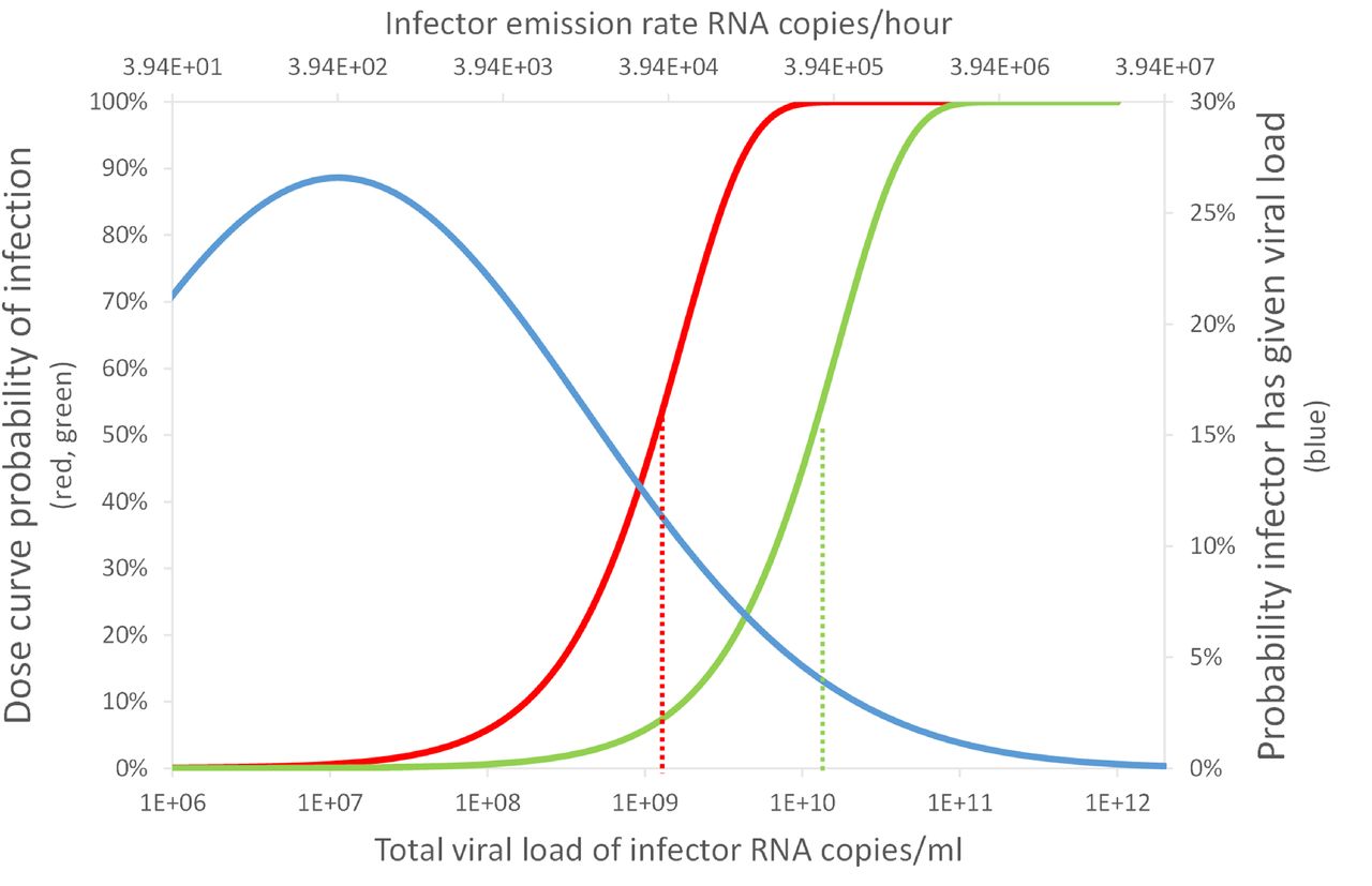
An indication of the relationship between the viral load, L, and the consequent probability of infection, P (R), in the Big Office (green) and Small Office (red) for a susceptible occupant, and the probability of a single infected person having a viral load, P (L), (blue). Dashed vertical lines indicate the viral load required for P (R) = 50%.
The dose can be used to estimate a probability of infection using a doseresponse curve. However, there is no dose-response curve for SARS-CoV-2. A number of studies [21, 16, 22] apply a dose curve for the SARS-CoV-1 virus, which is a typical dose curve for corona viruses, and so it is applied here. There are obvious problems with this extrapolation and they are discussed in Section 5.5. The probability of infection of an individual person, P (R), is given by
 where, k is the reciprocal of the probability that a single pathogen initiates an infection. We use a value of k = 410 following DeDiego et al.[23].
2.2. Individual risk
A Relative Exposure Index (REI) is used to compare exposure risk for an individual person between two spaces following Jones et al. [15]. Here, the REI is the ratio of the dose, D, received by a susceptible occupant in each of two spaces using Equation 1 where the reference space is the denominator and the comparator space is the numerator. An advantage of using an REI is that uncertainty in the viral load of respiratory fluid (RNA copies per ml), which is used to determine the viral emission rate, G (RNA copies per m3), and the unknown dose response, cancels allowing scenarios to be compared. When the REI is > 1 the comparator space is predicted to pose a greater risk to an individual susceptible occupant because they inhale a larger dose in the comparator scenario, although the absolute risk that this dose will lead to a probability of infection is not considered. Any space that wishes to have a REI of unity or less, must at least balance the parameters in Equation 1.
2.3. Population infection risk
A limitation of the REI is that it does not consider the probability of encountering an infected person with the same viral load in each scenario. The probability that a number of infected people, I, is present in a space, P (I), with a number of people present, N, is determined by considering the community infections rate, C, and standard number theory for combinations.

The total number of transmissions that occur in a population, Nt, of Npop people, is the sum of the number of transmissions that occur in each transmission scenario.
For a large population, the number of people infected in each space can be given by the product of the number of susceptible people exposed, Ns, and the mean individual probability of infection for a scenario,  .
.

 where Ns(I) denotes the number of susceptible people exposed in spaces that contain I infected people, P (I) is the probability that a space contains I infected people, and Npop N −1 denotes the total number of spaces that occur when a population Npop is divided into groups of N people. Here, the proportion of the population who are infected can be given by

The exact solution for Equation 7 becomes increasingly difficult to evaluate as the space size increases. The calculation complexity is unlikely to be justified given the uncertainties in both the modelling assumptions and the available data. Therefore, simple approximations to the equation is desirable.
One approach is to express the number of transmission events using a single mean individual risk for all possible transmission scenarios. Here, the PPI can be expressed as
 where P (S) is the proportion of the population who are both exposed and susceptible, and
  is the average individiual infection risk that occurs in all potential transmission scenarios.
Transmission events can only occur when there are both one or more infected people present in a space (I > 0) and one or more susceptible people are present (I < N). It follows that the probability of a space containing a potential transmission event is given by

As the number of occupants tends to infinity, the probability that the space contains a potential transmission event approaches one, and is equal to zero for single occupancy spaces. This suggests that it may be better to partition a large space; see Section 1. Likewise, the probability that a space contains susceptible people can be minimised by reducing the community infections rate, as long as the community infections rate is less than half. Furthermore, each space contains (N − I) susceptible people in it. This allows the probability that a user of the space is both susceptible and exposed to be given by
 where P (S) approaches the proportion of susceptible people in the wider community as N → ∞.
Evaluating the mean individual risk is non-trivial. Here an approximation is used, where

Here P (L) is the probability of a person having a viral load L, and Ī denotes the mean number of infected people in a space that contains a potential transmission event, and is given by
This allows the proportion of people infected in a scenario to be approximated by
 and is further simplified by assuming that mean infection probabilities are adequately described using a mean viral load, which can often be found directly from the literature. Here
 where
where  is the mean dose received in the space where one infected personis present.
2.4. Scenarios
The probabilities given in Section 2.3 can be used to consider how the number of occupants may affect the relative exposure risk at population scale. First, we define a reference space against which others are compared. This space is an office, which is chosen because it is a common space that is well regulated in most countries and has consistent occupancy densities. It has an occupancy density of 10 m2 per person, a floor to ceiling height of 3 m, and an outdoor airflow rate of 10 l s−1 per person. There are 50 occupants who are assumed to be continuously present for 8 hours breathing for 75% and talking for 25%. Hereon it is known as the Big Office.
Then, we define a comparator space by subdividing the 50 person office into 10 identical spaces. Each space preserves the occupancy density, the per capita space volume, the outdoor airflow rate per person, and the air change rate. Hereon each comparator space is known as the Small Office.
All scenario inputs are given in Table 1.
Scenario inputs and calculations of individual risk.
2.5. Probabilistic estimates
To investigate overdispersion in the model we use a Monte Carlo approach that selects ten populations of 0.5×10⁶ people and divides them into an equal number of spaces, depending on the scenario; see Section 2.4. The predictions confirm the mathematics described herein, and identify the uncertainty in the number of transmissions that occur for each scenario; see Section 5.4. All inputs are given in Tables 1 and 2.
We do not explore uncertainty in other inputs because this has been done before [15] and to limit the exploration of uncertainty in the viral load and the community infection rate.
Scenario inputs and calculations of population risk.
3. Individual risk
The REI is the ratio of the dose predicted using Equation 1 for Big Office and Small Office; see Section 2.2. When the number of infected people and their respiratory activities, and the breathing rates of susceptible occupants, are identical in each space, the REI simplifies to a ratio of equivalent ventilation rates, ϕ V. The equivalent ventilation rate is used to determine the steady state concentration of viable virions. Table 1 shows that the removal rate ϕ is identical in both spaces and so the REI becomes a simple ratio of the number of occupants. This suggests that, in the presence of a single infected person, the relative risk is 10 times higher in the Small Office. This occurs because the Small Office contains ten times fewer people than the Big Office, and therefore the ventilation rate per infector is ten times smaller.
The equivalent ventilation rate per person, ϕ V N −1, is identical in both spaces and, if it is desirable to preserve the equivalent ventilation per person in two different spaces, the space volume per person must be preserved.
The removal rate, ϕ, includes the biological decay of the virus and the deposition of aerosols onto surfaces. Both of these removal mechanisms are space-volume dependent, and so their contribution to the removal of the virus is greater in spaces with a larger volume. Therefore, increasing the space volume per person also has the effect of reducing the REI. This has obvious physical limitations and a simpler approach is to reduce the number of people per unit of volume.
Equation 1 is used to calculate the dose of viable virions in each space and Table 1 shows that the magnitudes of the doses are small. There is great uncertainty in these values, attributable to modelling assumptions and in the inputs given in Table 1, but an increase of an order of magnitude still leads to a small dose. This fact is compounded by the value of unity for the viable fraction, which has the effect that all RNA copies inhaled are viable, which is unlikely. A viable fraction of unity was chosen because its true value is currently unknown, and this assumption simplifies the analysis. The value is clearly likely to be « 100% in reality, and so the actual doses would be substantially lower than those estimated here. This suggests that far-field transmission in buildings requires high viral emission rates, G, which are likely to be a rare event.
The probability of an infection occurring when a susceptible occupant is exposed to the dose reported in Table 1 is estimated using Equation 2 to be P (R) < 1% for both spaces and is approximately 10 times greater in the Small Office; see Table 2. Generally, this shows that the viral load has to be greater in the Big Office than in the Small Office to achieve the same P (R) when C < 1%. This is demonstrated by Figure 1, which describes the relationship between the viral load in respiratory fluid (RNA copies per ml) in each space attributable to any number of infected people and the consequent P (R) for a susceptible occupant, if the virus emission rate is assumed to be linearly related to the viral load of the infected person.
For any viral load, L, the dose is calculated using Equation 1, and the probability that it leads to an infection is calculated using Equation 2. This creates a dose-response curve for both scenarios where factors that influence the REI and, therefore, the dose, determine the viral loads necessary to lead to a specific probability of infection. It also shows the relationship between the viral load and the probability that a single infector has that viral load, P (L). The dashed vertical lines show the viral load required to give a 50% probability that the dose will lead to an infection for each scenario, P (R) = 50%. The area under the blue curve to the right of each vertical line is the probability that the viral load of the infected person leads to P (R) ≥ 50%. The probability is much smaller for the Big Office, which has the lower REI. This probability that an infected person has a viral load that leads to P (R) ≥ 50% is small, suggesting that the most likely outcome is P (R) ≤ 50%. There is great uncertainty in the magnitude of these values, particularly in P (R) and in the conversion of a viral load to a virus emission rate (see Section 2), but significant increases in them do not change the general outcomes of the analysis. More generally, increasing the number of occupants in a space while preserving the per capita volume has the effect of moving the P (R) curve to the right in Figure 1 and towards the tail of the P (L) curve, which reduces the likelihood of a sufficient viral load in the space.
The P (L) distribution curve could be flattened and shifted to the left of Figure 1 by reducing the viral load of the infected population; for example, vaccination is shown to clear the virus from the body quicker in infected vaccinated people, which at a population scale could flatten the distribution of P (L) [24]. However, different variants of the SARS-CoV-2 virus could increase the viral load, or the proportion of viable virions, or the infectivity of virions, and move the curve to the right of Figure 1 [25, 26]. Other respiratory viruses will have different distributions of the viral load but the principles described here can be applied to them too.
4. Population risks
The analysis in Section 3 is underpinned by the assumption that there is a single infected person in each space. When the community infection rate (C) is known, Equation 3 can be used to estimate the probability that a specific number of infected people are present. When C = 1%, in the Big Office P (I = 0) is 61%, P (I = 1) is 31%, and P (I > 1) is 9%. For the Small Office, P (I = 0) is 95%, P (I = 1) is 5%, and P (I > 1) is negligible. This shows that the Big Office is over 12 times more likely to have an infected person present than the Small Office, although Table 1 shows that the relative risk is 10 times smaller in the Big Office than the Small Office when a single infected person is present. However, it is much more likely that both spaces do not have an infected person present, but when they are, the most likely number of infected people is 1. The mean number of infected people is just over 1 in both spaces when C = 1%; see Equation 12.
Figure 1 shows the relationship between the probability of infection and the probability of a person having a particular viral load. The viral load that leads to an infection can be attributed to any number of infected people, but the probability of having more than 1 infected person in a space is generally small; see Equation 9. When only 1 infected person is assumed to be present, Figure 1 also shows that the most probable viral loads do not lead to a dose that leads to an infection in either the Small Office or the Big Office. Therefore, the infected person must have a significant viral load to infect susceptible occupants, which is an improbable event. The infection risk for susceptible occupants is lower in the Big Office than the Small Office when only 1 infected person is assumed to be present.
Bigger spaces that preserve the per capita volume given in Table 1, and where N » 50, have a higher probability of susceptible people, P (S), and infected people, P (0 < I < N). The effect on the aerosol concentration and the dose depends on the space volume per infected person, V I−1, relative to that of the Reference Space, the Big Office. If V I−1 decreases, then the aerosol concentration, the dose, and the probability of infection, P (R), all increase. Accordingly, spaces with a high volume per occupant have a lower infection risk. Here, spaces with high ceilings or low occupancy densities are advantageous.
An increase in C also increases the probabilities of the presence of infected people, P (0 < I < N), and susceptible people, P (S), in any space. This increases the total viral load, the dose, D, and the probability of infection, P (R). Accordingly, maintaining a low community infection rate is important. It is worth noting that C may vary by region where the occupants are from, or by a particular population demographic [27]. Then, it is appropriate to use C for that demographic, rather than using a national value. It is possible to assess C by taking randomised samples from the population, such as the UK Coronavirus (COVID-19) Infection Survey [28], which includes all infected people at all stages of the disease. However, this survey includes symptomatic people who are likely to be isolating and so the actual C is likely to be lower.
The information in Figure 1 can be combined to determine the total proportion of people infected, PPI, in a space for all viral loads as a function of the probability that an individual person has a particular viral load, P (L), the probability of the risk of infection, P (R), the probability of the presence of susceptible people P (S), and the average number of infected people, Ī.
Figure 2 shows the proportion of people infected and the total viral load (see Equation 15) where the area under each curve is the proportion of the entire population infected for a community infection rate of C = 1%, and assuming that two equal populations, one distributed evenly across a number of Small Office scenarios and the other distributed evenly across a number of Big Office scenarios. Figure 2 indicates that the probability of far-field infection is PPI = 0.43% in the Small Office and PPI = 1.59% in the Big Office, which shows that the risk is 3 to 4 times higher in the Big Office. The absolute values are likely to be much smaller than those calculated here because of the conservative assumptions used to estimate the viral emission from viral load (see Section 2.1), so the PPI may well be « 1% in both spaces using less conservative assumptions; see the Supplementary Materials1. This indicates that although there are benefits of subdividing for a population, their magnitude needs to be considered against other factors, such as the overall work environment, labour and material costs, and inadvertent changes to the ventilation system and strategy.

An indication of the relationship between the proportion of a population infected for a particular viral load when the community infection rate is C = 1%. The area under the curve represents the total proportion of people infected for the Small Office (red) and the Big Office (green).
A transmission ratio, TR, gives an indication of relative risk of infection where

Here, the TR is 0.27.
The uncertainties in all of the values given here are significant and so it is not possible to be confident in the magnitude of the PPI or the TR, but testing the model with a range of assumptions enables an assessment of general trends; for example, how increasing occupancy and preserving per capita space volume and ventilation rates impact the risk of infection and how different mitigation measures, such as increasing the ventilation rate, affect the relative PPI. These are discussed in Section 5.
5. Discussion
5.1. Ventilation and space volume
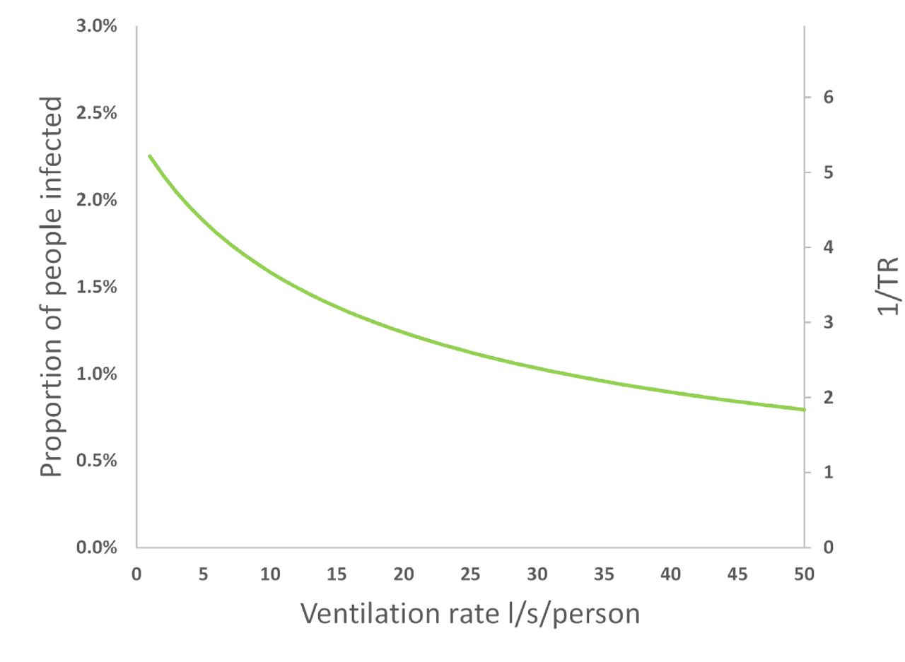
The quotient of the proportion of people infected in the two scenarios gives a Transmission Ratio, TR, see Equation 16. Increasing the per capita ventilation rate, ψV N −1, or space volume, V N −1, in the Big Office reduces the inverse of the TR. This has the effect of increasing the total removal rate, ϕ, and reducing the dose and the probability of infection; see Equation 1 and Figure 3. However, there is a law of diminishing returns in reducing the PPI by increasing the ventilation rate because the dose is inversely proportional to ϕ. Therefore, it is more important to increase the ventilation rate in a poorly ventilated space than in a well ventilated space because the change in the PPI is greater.

The effect of increasing the per capita ventilation rate, ψV N −1, in the Big Office on the PPI and the TR when the per capita ventilation rate in the Small Office is a constant 10 l s−1 per person. All values are illustrative.
A similar effect is seen when increasing the per capita space volume in the Big Office while maintaining a constant per capita ventilation in both spaces. This is because the dose is inversely proportional to volume. Furthermore, the product of the space volume and the total removal rate, ϕ V, is proportional to the concentration of the virus in the air and, therefore, the dose. The per capita ventilation rate is constant in both spaces and so the air change rate in the Big Office decreases as its volume increases. However, this reduction is offset by the surface deposition and biological decay rates, which remain constant and have a greater effect on the value of the equivalent ventilation rate, ψV, as the space volume increases; see Section 2.1.
Equation 1 assumes a steady-state concentration of the virus has been reached based on the assumption that the exposure time, T, is significant. However, the time taken to reach the steady-state concentration in large spaces may be significant and affects the dose over shorter exposure periods. This is an example of the reservoir effect, the ability of indoor air to act as a fresh-air reservoir and absorb the impact of contaminant emissions. The greater the space volume, the greater the effect. These factors highlight the benefits of increasing the per capita space volume.
5.2. Occupancy
Figure 4 shows the effect of increasing the number of occupants in the Big Office while maintaining both the per capita space volume, V N −1, and ventilation rate, ψV N −1. As the number of occupants increases, the PPI increases at an ever diminishing rate because the magnitude of the equivalent ventilation rate, ϕ V, increases at a greater rate than the probability of the mean number of infected people, Ī.

The effect of increasing the occupancy in the Big Office, where the space volume per person and ventilation rate per person is fixed at 30 m3 and 10 l s−1 respectively, on the PPI (green) and TR (black). All values are illustrative.
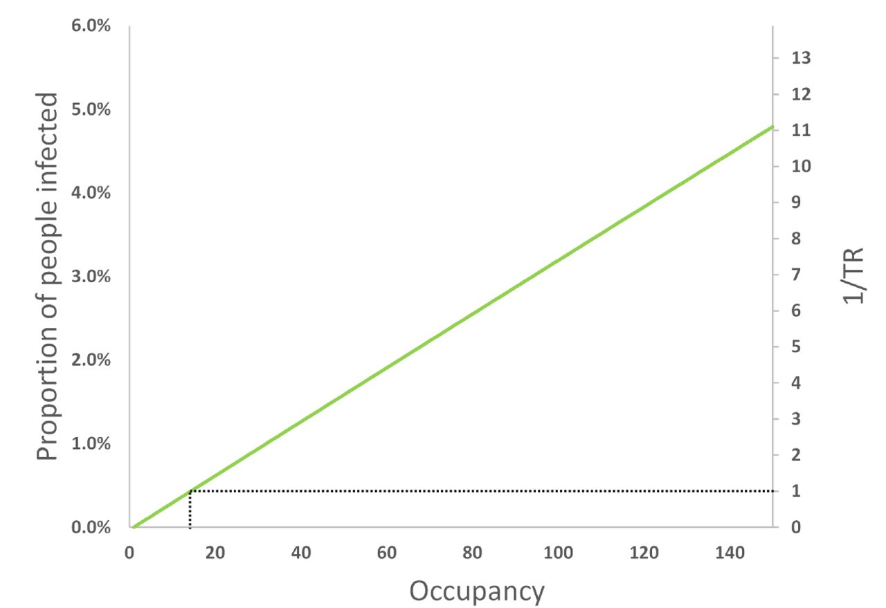
However, if the volume and ventilation rate remain constant as the occupancy increases, Figure 5 shows that the PPI and the inverse of the TR increase linearly with occupancy. Here, the total removal rate, ϕ, remains constant but the per capita space volume and ventilation rate reduce. Therefore, the Big Office could have 14 occupants and have the same PPI as the Small Office occupied by 5 people. Extrapolating to two identical populations of 140 people split into 28 Small Offices with 5 people in each, and 10 Big Offices with 14 people in each, the same PPI can be achieved.

The effect of increasing the occupancy in the Big Office where the space volume and ventilation flow rate is fixed for a designed occupancy of 50 people (1500 m3 and 500 l s−1, respectively), on the PPI and TR. All values are illustrative.
This suggests that reducing the number of occupants in a space is the most effective means of reducing the inverse of TR towards unity. To achieve the same goal by increasing the ventilation rate or the per capita space volume would require unfeasibly large increases in both.
5.3. Community infection rate
Figure 6 shows that the community infection rate, C, has a significant effect on the PPI and the TR. This is because it affects both the probability of a viral load, P (L), and the probability of having susceptible people in a space, P (S); see Equation 10. When C > 1%, the probability of transmission increases dramatically, suggesting that it strongly influences the spread of the virus indoors. Figure 6 also shows that C only affects the TR when the number of occupants, N, is less than the reciprocal of the community infection rate, N < 1/C. Thereafter, the TR is constant irrespective of the community infection rate; see the Supplementary Materials4.

The effect of increasing the community infection rate, C, on the PPI in the Big Office (green) and the Small Office (red) and on the TR (black). All values are illustrative.
5.4. Overdispersion
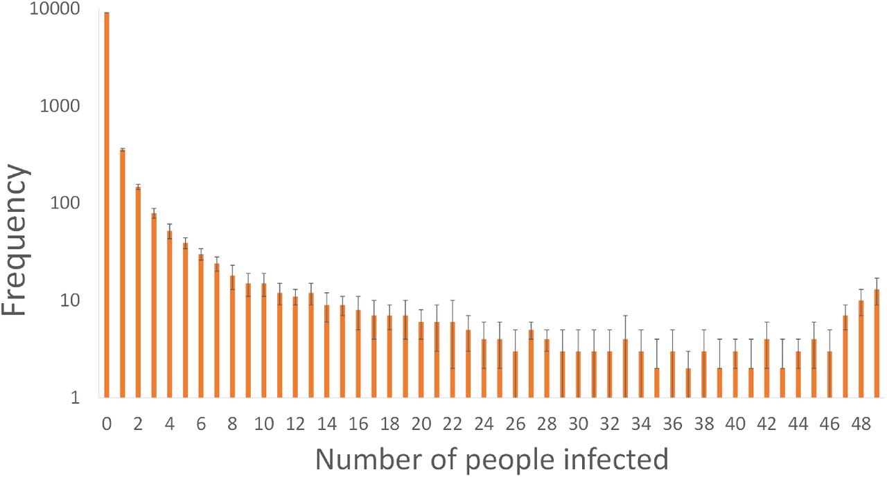
The Monte Carlo approach described in Section 2.5 was used to interrogate every scenario and estimate the number of susceptible people infected when an infected person is present in the Big Office. The Monte Carlo predictions indicate that at least one infected person was present 39% of the time, confirming the value of P (S) given in Table 2 determined using Equation 9. But, it also indicates that there was no transmission in 90% of the scenarios. When a transmission does occur, the most common outcome is a single transmission event; see Figure 7. This indicates that the dose inhaled by all susceptible people is usually small enough not to lead to an infection. At least 40 susceptible occupants are infected in the Big Office only 0.5% of the time, given the assumptions in Table 1. This suggests that so called super-spreader events are rare; see Figure 7. This distribution reflects the overdispersion of transmission recorded for SARS-CoV-2 and, although this work only considers one transmission route, similar relationships between the viral load and the number of transmission events may also be true for other transmission routes [11, 29, 30, 31, 32].

Uncertainty in the number of susceptible people infected in the Big Office Scenarios estimated using a Monte Carlo approach.
Applying the MC approach to the Small Office shows that the overdispersion is less pronounced because there are fewer susceptible people, which limits the number of people who can be infected when an infected person has a high viral load. Here, 0.2% of all scenarios, and 25% of scenarios with at least one transmission, had 4 infections of susceptible people. In the Small Office, all 4 susceptible occupants were infected in 46% of scenarios where at least one person was infected.
There are very few epidemiological examples of high secondary COVID-19 transmission events where > 80% of occupants in a scenario are infected and this suggests that our assumptions over-estimate the viral emission rate. One reason is the assumption that all genome copies are viable virions, which is very unlikely.
Figure 7 shows that the frequency of the number of susceptible people infected is highest at zero and decreases as the number of susceptible people infected increases. However, the frequency later increases as the number of susceptible people infected approaches the number of occupants. This reflects the shape of the probability of infection curve in Figure 1 where a point is reached when the viral load leads to the infection of all susceptible people, and a higher viral load cannot infect more people. The phenomena is a function of occupancy and is less likely to occur as the number of occupants increases because the viral load required to infect all susceptible people increases, assuming that the per capita space volume and ventilation rate are constant.
5.5. Limitations
Some limitations and uncertainties in this work have already been addressed, particularly those concerning the viral load and the dose-response relationship. However, there are a number of other aspects that increase uncertainty in it. Firstly, the models assume homogenous instantly mixed indoor air to simplify the estimate of a dose. This assumption is unlikely to be true in some spaces, especially in large spaces where the concentrations of virions in the air is likely be a function of the distance from the infected person. It is unclear at which space volume this assumption becomes less useful, but it is likely to be a few thousand cubic metres.
The approach described in Section 2 only considers the far-field transmission of virus, and not near-field transmission, which is likely to be the dominant route of transmission. The concentration of the virus in aerosols and droplets per unit volume of air is several orders of magnitude greater closer to the infected person at distances of < 2 m [3, 9]. However, it is likely that the method of calculating the probability of viral load of infected people, P (L), is also important for the dose received by near-field transmission and should be explored further in the future.
The distribution of viral load of an infected person around the median will affect the probability of transmission. We apply a log-normal distribution, see Section 2, but another, such as the Weibull distribution, will affect the transmission probabilities differently.
The model also assumes a naïve population of susceptible people, and it is unclear whether a higher infective dose is required for susceptible people who have a greater immune response obtained from vaccination or a previous infection. This paper does not consider the effect of the magnitude of the dose on subsequent disease severity. However, a recent review suggests that it is highly unlikely there is a link between dose and disease severity [33].
There is uncertainty in the dose-response relationship and the proportion of people infected. In the absence of knowledge, we have assumed that the dose-response curve for SARS-CoV-1 also applies to SARS-CoV-2; see Section 2.1. The SARS-CoV-1 dose-response curve was generated from four groups of inoculated transgenic mice [23] that were genetically modified to express the human protein receptor of the SARS-CoV-1 virus. In three of the groups all mice were infected and in the fourth one-third were infected. The dose-response curve was fitted to data from these four groups and, although it is limited, it is sufficient to assume that the curve follows the exponential distribution rather than the Beta-Poisson distribution. A further limitation is that the response of humans to a dose of SARS-CoV-1 may vary significantly from that of transgenic mice. For a further discussion, see the Supplemental Material4. There is also uncertainty in the measurement of the viral load used to challenge the study, and whether or not dose curves are valid for predicting low probabilities of infection at very low virus titres. Other studies have used alternative dose-response curves for other coronaviruses, all of which have similar uncertainties [21, 16].
The viral load of an infected person is the number of RNA copies per ml of respiratory fluid, whereas the viral emission is the amount of RNA copies per unit volume of exhaled breath; see Section 2.1. It has been established that the viral load of an infected person increases in time from the moment of infection and is highest just before, or at, the onset of COVID-19 symptoms. As COVID-19 progresses the viral load reduces, normally within the first week after the onset of symptoms [34, 35]. The viral load also varies between people at any stage of the infection, which increases uncertainty in it [36, 37, 38, 19, 39, 18].
The viral load can be inferred from the cycle threshold values of real time reverse transcription quantitative polymerase chain reaction (RT qPCR) nasopharyngeal (NP) swabs. This method assumes a direct correlation between the viral load of a swab and the viral load of respiratory fluid [40, 12]. RT qPCR is a semi-quantitative method because it requires a number of amplification cycles to provide a positive signal of the SARS-CoV-2 genome, which is proportional to the initial amount of viral genome in the original sample. The cycle threshold is the number of polymerase chain reaction cycles that are required before the chemical luminescence is read by the equipment. The lower the starting amount of viral genome, the greater the number of amplification cycles required. A calibrated standard curve is then used to estimate the starting amount of viral genomic material. However, the standard curve varies between test assays (investigative procedures) and different RT qPCR thermal cyclers, the laboratory apparatus used to amplify segments of RNA. This method also assumes a complete doubling of genetic material after each cycle. The exponential relationship means that errors in the calculation of the initial quantity of genomic material are orders of magnitude higher for for low cycle counts than for high cycle counts. Additionally, if genomic data is taken from NP swabs, the estimated concentration of genomic material per unit volume is often related to the amount of genomic material in the buffer solution2 in which NP swabs are eluted and used in the assay, and not necessarily to the amount in a patient’s respiratory fluid. The amount of genomic material added to the buffer solution is dependent on both a patient’s viral load and the quality of the collection of the NP sample, which is highly variable. Therefore, it is not possible to determine absolute values of the viral load in a patient’s respiratory fluid using this method. However, data collected in this way is indicative of a range of variability, much of which is likely to be proportional to the viral load of the person at the time the sample was collected. Some recent data suggests that the viral load of NP swabs may not reflect the amount of infectious material present [19]. However, it is important to note that there are wide variations in the measured genomic material in NP swabs and that the viral load in respiratory fluid is likely to vary by several orders of magnitude.
There is clearly uncertainty in the viral load of respiratory fluid. There is also uncertainty in the viral concentration in respiratory aerosols and droplets and the distribution is currently unclear. Some studies suggest that the number of virions in small aerosols with a diameter of < 1 μm is higher than would be expected given the viral concentration in the respiratory fluid [41, 42] and that for SARS-CoV-2 there may be more genomic material in the smallest aerosols [43].
There is high variability between people in the total volume of aerosols generated per unit volume of exhaled breath, and it is dependent upon the respiratory activity, such as talking and singing, and the respiratory capacity [44, 45, 46, 47]. Coleman et al. [43] show that SARS-CoV-2 genomic material is detectable in expirated aerosols from some COVID-19 patients, but not all of them because 41% exhaled no detectable genomic material. Singing and talking generally produce more genomic material than breathing, but there is large variability between patients. This suggests that respiratory activities that have previously been shown to increase aerosol mass also increase the amount of viral genomic material emitted. However, the viral concentration in aerosols cannot be determined because the study did not measure the mass of aerosols generated. Coleman et al. also show that the variability in the amount of genomic material measured in expirated aerosols is consistent with the variability of viral loads determined using swabs and saliva [43].
Similarly, Adenaiye et al. [48] detected genomic material in aerosols from patients infected with SARS-CoV-2 who provided a sample of exhaled air when talking or singing. Genomic material was more frequently detected in exhaled aerosols when the viral load of saliva or mid-turbinate swabs was high; > 108 and > 106 RNA copies for mid-turbinate swabs and saliva samples, respectively. Furthermore, they were able to culture viable virus from < 2% of fine aerosol samples. It should be noted that one positive sample was from a culture developed from a fine aerosol sample that had an amount of genomic material that was less than the detection limit of the qRT PCR method and so could be an artefact. Nevertheless, this provides some evidence to support the epidemiological evidence that viable virus can exist in exhaled aerosols.
Miller et al. suggests that around 1 : 1000 genome copies are likely to be infectious virion [49, 12]. Adenaiye et al. use mid-turbinate swabs to estimate that there are around 1 : 104 viable virus per measured genome copies[48]. We make the assumption that all genome copies are viable virion, which either over-estimates their infectiousness when using the Coleman et al. data, or is similar to the assumption of Miller et al. if the viable virion emission rate is in the order of 1000 virions per hour; see Appendix Appendix A.
6. Conclusions
The number of occupants in a space can influence the risk of far-field airborne transmission that occurs at distances of > 2 m because the likelihood of having infectious and susceptible people both scale with the number of occupants. Therefore, mass-balance and dose-response models are applied to determine if it is advantageous to sub-divide a large reference space into a number of identical smaller comparator spaces to reduce the transmission risk for an individual person and for a population of people.
The reference space is an office with a volume of 1500 m3 occupied by 50 people over an 8 hour period, and has a ventilation rate of 10 l s−1 per person. The comparator space is occupied by 5 people and preserves the occupancy period and the per capita volume and ventilation rate. The dose received by an individual susceptible person in the comparator Small Office, when a single infected person is present, is compared to that in the reference Big Office for the same circumstances to give a relative exposure index (REI) with a value of 10 in the Small Office. This REI is a measure of the risk of a space relative to the geometry, occupant activities, and exposure times of the reference scenario and so it is not a measure of the probability of infection. Accordingly, when a single infected person is assumed to be present, a space with more occupants is less of a risk for susceptible people because the equivalent ventilation rate per infected person is higher.
The assumption that only one infected person is present is clearly problematic because, for a community infection rate of 1%, the most likely number of infected people in a 50 person space is none. A transmission event can only occur when there are both one or more infected people present in a space and one or more susceptible people are present. The probability of a transmission event occurring increases with the number of occupants and the community infection rate; for example, the Big Office is over 12 times more likely to have infected people present than the Small Office. However, the geometry and ventilation rate in a larger space are non-linearly related to the number of infected and susceptible people and so their relationship with the probability of a transmission event occurring is also non-linear. These effects are evaluated by considering a large population of people. But, this introduces uncertainty in factors that vary across the population, such as the viral load of an infected person, defined as the number of RNA copies per ml of respiratory fluid. The viral load varies over time and between people at any stage of the infection.
By applying a distribution of viral loads across a population of infected people, secondary transmissions (new infections) are found to be likely to occur only when the viral load is high, although the probabilities of this occurring in the Big Office and the Small Office are low. This makes it hard to distinguish the route of transmission epidemiologically. Generally, the viral load must be greater in the Big Office than in the Small Office to achieve the same proportion of the population infected when the community infection rate is ≤ 1%. The viable fraction is unknown but a value of unity was chosen for computational ease, yet the estimated doses and infection probabilities are small. Therefore, it is likely that far-field transmission is a rare event that requires a set of Goldilocks conditions that are just right.
There are circumstances where the magnitude of the total viral load of the infected people is too high to affect the probability of secondary transmissions by increasing ventilation and space volume. Conversely, when the total viral load is very small the dose is too low to lead to an infection in any space irrespective of its geometry or the number of susceptible people present. There is a law of depreciating returns for the dose and, therefore, the probability of infection, and the ventilation rate because they are inversely related. Accordingly, it is better to focus on increasing effective ventilation rates in under-ventilated spaces rather than increasing ventilation rates above those prescribed by standards, or increasing effective ventilation rates using air cleaners, in already well-ventilated spaces.
There are significant uncertainties in the modelling assumptions and the data used in the analysis and it is not possible to have confidence in the calculated magnitudes of doses or the proportions of people infected. However, the general trends and relationships described herein are less uncertain and may also apply to airborne pathogens other than SARS-CoV-2 at the population scale. Accordingly, it is possible to say that there are benefits of subdividing a population, but their magnitudes need to be considered against other factors, such as the overall working environment, labour and material costs, and inadvertent changes to the ventilation system and strategy. However, it is likely that the benefits do not outweigh the costs in existing buildings when a less conservative viable fraction is used because it decreases the magnitude of the benefits significantly. It is likely to be more cost-effective to consider the advantages of partition when designing new resilient buildings because the consequences can be considered from the beginning.
There are other factors that will reduce the risk of transmission in existing buildings. Local and national stakeholders can seek to maintain low community infection rates, detect infected people with high viral loads using rapid antigen tests and isolate them (see the Supplementary Materials3), reduce the variance and magnitude of the viral load in a population by encouraging vaccination. Changes can be made to the use of existing buildings and their services, such as reducing the occupancy density of a space below the level it was designed for while preserving the magnitude of the ventilation rate, reducing exposure times, and ensuring compliance with ventilation standards.
Data Availability
All data produced in the present work are contained in the manuscript and Supplemental Materials
Acknowledgements
The authors acknowledge the Engineering and Physical Sciences Research Council (EP/W002779/1) who financially supported this work. They are also grateful to Constanza Molina for her comments on this paper.
Appendix A. Estimating viral emission from viral load
We assume that the RNA copies per ml concentration is constant in aerosols and in NP swabs and then we use the assumptions of Jones et al. [15] to convert a NP viral load into a virus emission rate. This method follows Jones et al. and is derived from the work of Morawskwa et al. who determine volume distribution aerosols for different respiratory activities, and is similar to that used by Lelieveld et al. [15, 17, 47]. Table A.3 shows the estimated virus emission rate for different respiratory activities when the viral load is 107 RNA copies per ml. For comparison, median measured values of virus emission in aerosols from Coleman et al. are given. These values were measured by collecting RNA copies from COVID-19 patients, where the median cycle threshold, required to process diagnostic samples, was 16. [43].
Estimated emission rates from an infected person with a viral load of 107 RNA copies per ml compared to measured emission rates from patients with a median cycle threshold of 16 [43]
Additionally, unpublished work by Adenaiye et al. measured viral genome in patients infected by the SARS-CoV-2 alpha variant, who were breathing and talking, in coarse (> 5 μm) and fine (≤ 5 μm) aerosols with a total geometric mean of 1440 RNA copies h−1 and a maximum of 3×10⁵ RNA copies h−1 [48]. These are greater than the estimated values given in Table A.3, but the viral load, measured by genome copies from mid-turbinate swabs, was generally orders of magnitude higher than 107 RNA copies per ml.
In Section 4, the inhaled dose is calculated for all possible viral loads. Here, it should be noted that the calculated RNA copies emission rate is assumed to be linearly related to the viral load of respiratory fluids, so that a viral load of 108 RNA copies per ml has a ten-fold greater emission rate. For comparison, a virus emission rate of 394 RNA copies h−1 (assumed for a viral load of 107 RNA copies per ml) leads to an individual doses of around RNA copies and 0.2 RNA copies for the Small Office and Big Office scenarios, respectively.
The calculated emission rate of viral genome for a viral load of 107 RNA copies per ml is a reasonable fit to the Coleman et al. and Adenaiye et al. data. For further details see the Supplementary Materials4.
Footnotes
Nomenclature
- Ī
- mean number of infected people present

- mean dose in a space where one infected personis present
- Ī
- mean number of infected people in a space that contains a potential transmission event
- mean individual probability of infection occurring in a scenario
- mean individual infection risk that occurs in all potential transmission scenarios
- ϕ
- total removal rate (s−1)
- C
- community infections rate (%)
- D
- dose (viable virions)
- G
- emission rate of RNA copies (RNA copies s−1)
- I
- number of infected people
- K
- fraction of aerosol particles absorbed by respiratory tract
- k
- reciprocal of the probability that a single pathogen initiates an infection
- L
- viral load (RNA copies per ml of respiratory fluid)
- N
- number of occupants
- Ns
- number of susceptible people exposed
- Ns(I)
- number of susceptible people exposed in spaces that contain I infected people
- Nt
- number of transmissions in the entire population
- Nt(I)
- number of transmissions that occur in spaces that contain I infected people
- Npop
- population size
- P (0 < I < N)
- probability of a space containing a potential transmission
- P (I)
- probability of I infected people present
- P (L)
- probability of a viral load
- P (R)
- individual probability of infection
- P (S)
- probability of a person being both susceptible and exposed to the virus
- qsus
- susceptible person respiratory rate (m3 s−1)
- T
- exposure period (s)
- V
- space volume (m3)
- υ
- viable fraction


References


