
Abstract
With age, eyesight declines and the vulnerability to age-related eye diseases such as glaucoma, cataract, macular degeneration and diabetic retinopathy increases. With the aging of the global population, the prevalence of these diseases is projected to increase, leading to reduced quality of life and increased healthcare cost. In the following, we built an eye age predictor by training convolutional neural networks to predict age from 175,000 eye fundus and optical coherence tomography images (R-Squared=83.6+-0.6%; root mean squared error=3.34+-0.07 years). We used attention maps to identify the features driving the eye age prediction. We defined accelerated eye aging as the difference between eye age and chronological age and performed a genome wide association study [GWAS] on this phenotype. Accelerated eye aging is 28.2+-1.2% GWAS-heritable, and is associated with 255 single nucleotide polymorphisms in 122 genes (e.g HERC2, associated with eye pigmentation). Similarly, we identified biomarkers (e.g blood pressure), clinical phenotypes (e.g chest pain), diseases (e.g cataract), environmental variables (e.g sleep deprivation) and socioeconomic variables (e.g income) associated with our newly defined phenotype. Our predictor could be used to detect premature eye aging in patients, and to evaluate the effect of emerging rejuvenation therapies on eye health.
Background
Aging affects all components of the eye (eyelids, lacrimal system, cornea, trabecular mesh work, uvea, crystalline lens, retina, macula 1) and is associated with the onset of age-related eye diseases such as presbyopia, cataract, glaucoma, macular degeneration and retinopathy 2 leading to reduced quality of life, increased healthcare costs 3, and shortened lifespan due to the increased risk for falls 4.
Eye age predictors have been built to study eye aging. Machine learning algorithms are trained to predict the age of the participant (also referred to as “chronological age”) from eye phenotypes and the prediction of the model can be interpreted as the participant’s eye age (also referred to as “biological age”). Accelerated eye aging is defined as the difference between eye age and age. Age has for example already been predicted from fundus 5, 6, iris 7–9 and eye corner images 10. Identifying the genetic and non-genetic factors underlying accelerated eye aging however remains an elusive question. Additionally, age has, to our knowledge, never been predicted from optical coherence tomography images [OCT].
In the following, we leverage 175,000 OCT and eye fundus images (Figure 1B), along with eye biomarkers (acuity, refractive error, intraocular pressure) collected from 37-82 year-old UK Biobank 11 participants (Figure 1A), and use deep learning to build eye age predictors. We perform a genome wide association study [GWAS] and an X-wide association study [XWAS] to identify genetic and non-genetic factors (e.g biomarkers, phenotypes, diseases, environmental and socioeconomic variables) associated with eye aging. (Figure 1C)

Legend for A - * Correspond to eye dimensions for which we performed a GWAS and XWAS analysis
Results
We predicted chronological age within approximately three years
We leveraged the UK Biobank, a dataset containing 175,000 eye fundus and OCT images (both left and right eyes, so approximately half fewer samples, Figure 1A and B), as well as eye biomarkers (acuity, intraocular and autorefraction tests) collected from 97,000-135,000 (Figure 1A and B) participants aged 37-82 years (Fig. S1). We predicted chronological age from images using convolutional neural networks and from scalar biomarkers using elastic nets, gradient boosted machines [GBMs] and shallow fully connected neural networks. We then hierarchically ensembled these models by eye dimension (Figure 1A and C).
We predicted chronological age with a testing R-Squared [R2] of 83.6+-0.6% and a root mean square error [RMSE] of 3.34+-0.07 years (Figure 2). The eye fundus images outperformed the OCT images as age predictors (R2=76.6+-1.3% vs. 70.8+-1.2%). The scalar-based models underperformed compared to the image-based model (R2=35.9+-0.5). Between the different algorithms trained on all scalar features, the non-linear models outperformed the linear model (GBM: R2=35.8+-0.6%; Neural network R2=30.8+-2.4%; Elastic net: R2=25.0+-0.4%).

* represent ensemble models
We defined eye age as the prediction outputted by one of the models, after correction for the analytical bias in the residuals (see Methods). For example fundus-based eye age is the prediction outputted by the ensemble model trained on fundus images. If not specified otherwise, eye age refers to the prediction outputted by the best performing, all encompassing ensemble model.
Identification of features driving eye age prediction
In terms of scalar features, we best predicted eye aging with a GBM (R2=35.8±0.6%) trained on autorefraction (35 features), acuity (eight features) and intraocular pressure (eight features) measures, along with sex and ethnicity. Autorefraction measures alone predicted CA with a R2 of 29.0±0.2%, acuity measures with a R2 of 15.5±0.2% and intraocular pressure with a R2 of 6.9±0.1%. Specifically, the associated most important scalar features for the model including all the predictors are (1; 2) the spherical power (right and left eyes), (3; 4) the cylindrical power (right and left eyes), (5; 6) the astigmatism (right and left eyes), (7) the 3mm asymmetry index (left eye), (8) the 6mm cylindrical power (right eye), (9) the 3mm asymmetry angle (left eye) and (10) the 6mm weak meridian angle. In the linear context of the elastic net (R2=25.0±0.4%), the spherical power, the cylindrical power, the 6mm cylindrical power and the 6mm weak meridian angle are associated with older age, whereas the astigmatism angle, the 3mm asymmetry index and the 3mm asymmetry angle are associated with younger age.
In terms of eye fundus images, the Grad-RAM attention maps tended to highlight the eye regions that were highly vascularized, whereas the saliency maps also frequently highlighted the center of the eye (Figure 3). In terms of OCT images, Grad-RAM highlighted all the retinal layers with different regions emphasized for different participants. Similarly, saliency maps highlighted different layers for different participants, as well as the fovea. The resolution of the resized images makes it difficult to precisely identify these layers, but the list seems to include the posterior hyaloid surface, the inner limiting membrane, the external limiting membrane, ellipsoid portion of the inner segments, the cones outer segment tips line and the retinal pigment epithelium (Figure 4).
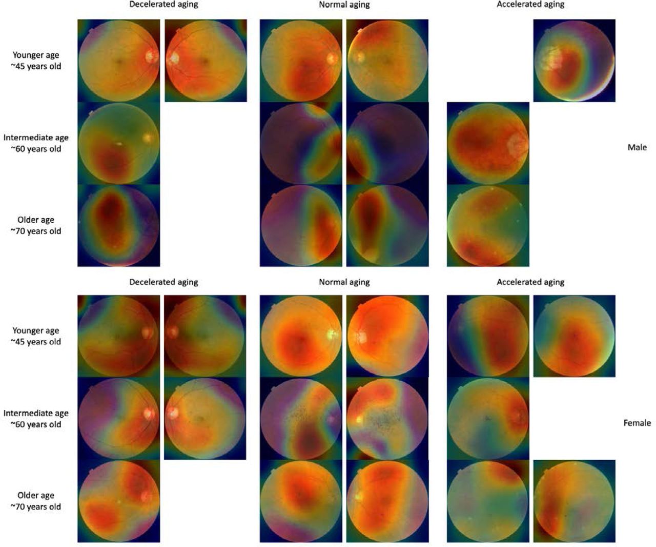
Warm filter colors highlight regions of high importance according to the Grad-RAM map. Missing images are left as a white space.

Warm colors highlight regions of high importance according to the Grad-RAM map.
Genetic factors and heritability of accelerated eye aging
We performed three genome wide association studies [GWASs] to estimate the GWAS-based heritability of general (h_g2=28.2±1.2%), fundus image-based (h_g2=26.0±0.9%), and OCT image-based (h_g2=23.6±0.9%) accelerated eye aging. We identified 255 single nucleotide polymorphisms [SNPs] in 122 genes associated with accelerated aging in at least one eye dimension. (Table 1 and Figure 5)
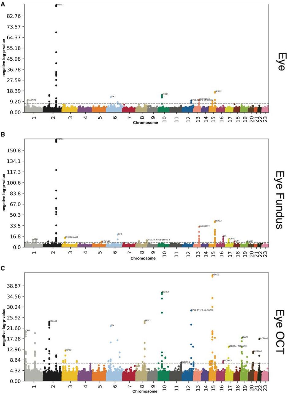
-log10(p-value) vs. chromosomal position of locus. Dotted line denotes 5x10⁻⁸.
GWASs summary - Heritability, number of SNPs and genes associated with accelerated aging in each eye dimension
We found that accelerated eye aging is 28.2±1.2% heritable and that 55 SNPs in 27 genes are significantly associated with this phenotype. The GWAS highlighted nine peaks: (1) H3YL1 (SH3 And SYLF Domain Containing 1, linked to Meier-Gorlin syndrome); (2) HERC2 (HECT And RLD Domain Containing E3 Ubiquitin Protein Ligase 2, associated with eye pigmentation); (3) HTRA1 (HtrA Serine Peptidase 1, involved in cell growth regulation); (4) COL4A4 (Collagen Type IV Alpha 4 Chain, a component of collagen that is only found in basement membranes 12); (5) TTK (TTK Protein Kinase, involved in mitotic checkpoint and linked to retinoblastoma); (6) SLC16A1 (Solute Carrier Family 16 Member 1, a monocarboxylate transporter); (7) LINC01072 (Long Intergenic Non-Protein Coding RNA 1072, a long intergenic non-coding RNA); (8) RDH5 (Retinol Dehydrogenase 5, involved in visual pigment synthesis and linked to Fundus Albipunctatus and Fundus Dystrophy); and (9) ABHD2 (Abhydrolase Domain Containing 2, Acylglycerol Lipase, linked to Retinitis Pigmentosa) 13.
We found that accelerated eye fundus-based aging is 26.0±0.9% heritable and that 109 SNPs in 44 genes are significantly associated with this phenotype. The ten highest peaks highlighted by the GWAS are (1) SH3YL1 (linked to Meier-Gorlin syndrome); (2) HERC2 (associated with eye pigmentation); (3) LINC01072 (a long intergenic non-coding RNA); (4) IRF4 (Interferon Regulatory Factor 4, involved in immune response to viruses); (5) ST3GAL6-AS1 (ST3GAL6 Antisense RNA 1, a long intergenic non-coding RNA); (6) PPL (Periplakin, present in keratinocytes); (7) PDE6G (Retinal Rod Rhodopsin-Sensitive CGMP 3’,5’-Cyclic, involved in the phototransduction signaling cascade of rod photoreceptors); (8) LGR6 (Leucine Rich Repeat Containing G Protein-Coupled Receptor 6, involved in GPCR signaling); (9) MACF1 (Microtubule Actin Crosslinking Factor 1, involved in actin-microtubules interactions); and (10) TCF4 (Transcription Factor 4, involved in corneal dystrophy) 13.
We found that accelerated eye OCT-based aging is 23.6±0.9% heritable and that 149 SNPs in 80 genes are significantly associated with this phenotype. The ten highest peaks highlighted by the GWAS are (1) ABHD2 (Abhydrolase Domain Containing 2, Acylglycerol Lipase, linked to Retinitis Pigmentosa.); (2) ARMS2 (Age-Related Maculopathy Susceptibility 2, a component of the eye’s choroidal extracellular matrix, linked to age-related macular degeneration and retinal drusen); (3) RDH5 (Retinol Dehydrogenase 5, involved in visual pigment synthesis and linked to Fundus Albipunctatus and Fundus Dystrophy); (4) RP1L1 (RP1 Like 1, a retinal-specific protein involved in photosensitivity and rod photoreceptors’ morphogenesis, and linked to Occult Macular Dystrophy and Retinitis Pigmentosa); (5) COL4A4 (Collagen Type IV Alpha 4 Chain, a component of collagen that is only found in basement membranes 12); (6) TTK (TTK Protein Kinase, involved in mitotic checkpoint and linked to retinoblastoma); (7) CFH (Complement Factor H, involved in innate immune response to microbial infections); (8) ZNF593 (Zinc Finger Protein 593, involved in transcriptional activity regulation); (9) OCA2 (OCA2 Melanosomal Transmembrane Protein, linked to iris pigmentation); and (10) APOC1 (Apolipoprotein C1, involved in high density lipoprotein (HDL) and very low density lipoprotein (VLDL) metabolism)13.
Biomarkers, clinical phenotypes, diseases, environmental and socioeconomic variables associated with accelerated eye aging
We use “X” to refer to all nongenetic variables measured in the UK Biobank (biomarkers, clinical phenotypes, diseases, family history, environmental and socioeconomic variables). We performed an X-Wide Association Study [XWAS] to identify which of the 4,372 biomarkers classified in 21 subcategories (Table S4), 187 clinical phenotypes classified in 11 subcategories (Table S7), 2,073 diseases classified in 26 subcategories (Table S10), 92 family history variables (Table S13), 265 environmental variables classified in nine categories (Table S16), and 91 socioeconomic variables classified in five categories (Table S19) are associated (p-value threshold of 0.05 and Bonferroni correction) with accelerated eye aging in the different dimensions. We summarize our findings for general accelerated eye aging below. Please refer to the supplementary tables (Table S5, Table S6, Table S8, Table S9, Table S11, Table S12, Table S17, Table S18, Table S20, Table S21) for a summary of non-genetic factors associated with general, fundus-based and OCT-based accelerated eye aging. The full results can be exhaustively explored at https://www.multidimensionality-of-aging.net/xwas/univariate_associations.
Biomarkers associated with accelerated eye aging
The three biomarker categories most associated with accelerated eye aging are urine biochemistry, blood pressure and eye intraocular pressure (Table S5). Specifically, 100.0% of urine biochemistry biomarkers are associated with accelerated eye aging, with the three largest associations being with microalbumin (correlation=.032), sodium (correlation=.027), and creatinine (correlation=.021). 100.0% of blood pressure biomarkers are associated with accelerated eye aging, with the three largest associations being with pulse rate (correlation=.075), systolic blood pressure (correlation=.044), and diastolic blood pressure (correlation=.040). 75.0% of eye intraocular pressure biomarkers are associated with accelerated eye aging, with the three largest associations being with right eye Goldmann-correlated intraocular pressure (correlation=.093), right eye corneal-compensated intraocular pressure (correlation=.092), and left eye Goldmann-correlated intraocular pressure (correlation=.090).
Conversely, the three biomarker categories most associated with decelerated eye aging are hand grip strength, spirometry and body impedance (Table S6). Specifically, 100.0% of hand grip strength biomarkers are associated with decelerated eye aging, with the two associations being with right and left hand grip strengths (respective correlations of .060 and .059). 100% of spirometry biomarkers are associated with decelerated eye aging, with the three associations being with forced expiratory volume in one second (correlation=.064), forced vital capacity (correlation=.060), and peak expiratory flow (correlation=.041). 100.0% of body impedance biomarkers are associated with decelerated eye aging, with the three largest associations being with whole body impedance (correlation=.040), left leg impedance (correlation=.038), and left arm impedance (correlation=.035).
Clinical phenotypes associated with accelerated eye aging
The three clinical phenotype categories most associated with accelerated eye aging are chest pain, breathing and general health (Table S8). Specifically, 100.0% of chest pain phenotypes are associated with accelerated eye aging, with the three largest associations being with chest pain or discomfort walking normally (correlation=.033), chest pain due to walking ceases when standing still (correlation=.030), and chest pain or discomfort (correlation=.030). 100.0% of breathing phenotypes are associated with accelerated eye aging, with the two associations being with shortness of breath walking on level ground (correlation=.059) and wheeze or whistling in the chest in the last year (correlation=.051). 62.5% of general health phenotypes are associated with accelerated eye aging, with the three largest associations being with overall health rating (correlation=.085), long-standing illness, disability or infirmity (correlation=.071), and falls in the last year (correlation=.032).
Conversely, the three clinical phenotype categories most associated with decelerated eye aging are sexual factors (age first had sexual intercourse: correlation=.030), mouth health (no mouth/teeth problems: correlation=.019) and general health (no weight change during the last year: correlation=.042). (Table S9)
Diseases associated with accelerated eye aging
The three disease categories most associated with accelerated eye aging are general health, cardiovascular diseases and eye disorders (Table S11). Specifically, 13.1% of general health variables are associated with accelerated eye aging, with the three largest associations being with personal history of disease (correlation=.039), problems related to lifestyle (correlation=.032), and presence of functional implants (correlation=.032). 11.7% of cardiovascular diseases are associated with accelerated eye aging, with the three largest associations being with hypertension (correlation=.061), chronic ischaemic heart disease (correlation=.030), and heart failure (correlation=.025). 11.4% of eye disorders are associated with accelerated eye aging, with the three largest associations being with cataract (correlation=.058),retinal disorders (correlation=.050), and retinal detachments and breaks (correlation=.041).
Conversely, the “diseases” associated with decelerated eye aging are related to pregnancy and delivery (perineal laceration during delivery: correlation=.029; single spontaneous delivery: correlation=.019; outcome of delivery: correlation=.044; supervision of high-risk pregnancy: correlation=.020). (Table S12)
Environmental variables associated with accelerated eye aging
The three environmental variable categories most associated with accelerated eye aging are sleep, smoking and physical activity (Table S17). Specifically, 57.1% of sleep variables are associated with accelerated eye aging, with the three largest associations being with napping during the day (correlation=.027), chronotype (being an evening person) (correlation=.026), and sleeplessness/insomnia (correlation=.026). 37.5% of smoking variables are associated with accelerated eye aging, with the three largest associations being with pack years adult smoking as proposition of lifespan exposed to smoking (correlation=.092), pack years of smoking (correlation=.090), and past tobacco smoking: smoked on most or all days (correlation=.066). 11.4% of physical activity variables are associated with accelerated eye aging, with the three largest associations being with time spent watching television (correlation=.063), no physical activity during the last four weeks among the ones listed in the questionnaire (correlation=.051), and types of transport used, work excluded: public transport (correlation=.042).
Conversely, the three environmental variable categories most associated with decelerated eye aging are physical activity, smoking and sleep (Table S18). Specifically, 57.1% of physical activity variables are associated with decelerated eye aging, with the three largest associations being with usual walking pace (correlation=.053), frequency of heavy do-it-yourself [DIY] work in the last four weeks (correlation=.046), and duration of heavy DIY (correlation=.044). 29.2% of smoking variables are associated with decelerated eye aging, with the three largest associations being with smoking status: never (correlation=.058), age started smoking (correlation=.057), and time from waking to first cigarette (correlation=.049). 28.6% of sleep variables are associated with decelerated eye aging, with the two associations being with snoring (correlation=.038) and getting up in the morning (correlation=.029).
Socioeconomic variables associated with accelerated eye aging
The three socioeconomic variable categories most associated with accelerated eye aging are sociodemographics (private healthcare: correlation=.020), social support (leisure/social activities: none of the listed: correlation=.021) and household (renting from local authority, local council or housing association: correlation=.043; type of accommodation: flat, maisonette or apartment: correlation=.032). (Table S20) Conversely, the three socioeconomic variable categories most associated with decelerated eye aging are social support, sociodemographics and household (Table S21). Specifically, 22.2% of social support variables are associated with decelerated eye aging, with the two associations being leisure/social activities: sports club or gym (correlation=.026) and being able to confide (correlation=.019). 14.3% of sociodemographic variables are associated with decelerated eye aging (one association: not receiving attendance/disability/mobility allowance. correlation=.048). 11.4% of household variables are associated with decelerated eye aging, with the three largest associations being with number of people in the household (correlation=.057), average total household income before tax (correlation=.054), and number of vehicles (correlation=.048).
Predicting accelerated eye aging from biomarkers, clinical phenotypes, diseases, environmental variables and socioeconomic variables
We predicted accelerated eye aging using variables from the different X-datasets categories (biomarkers, clinical phenotypes, diseases, environmental variables and socioeconomic variables). Specifically we built a model using the variables from each of their respective subcategories (e.g blood pressure biomarkers), and found that no dataset could explain more than 5% of the variance in accelerated eye aging.
Phenotypic, genetic and environmental correlation between fundus image-based and OCT image-based accelerated eye aging
Fundus image-based and OCT image-based accelerated eye aging are .239+-.005 correlated. For comparison purposes, the two convolutional neural networks architectures (InceptionV3 and InceptionResNetV2) trained on the exact same dataset yielded accelerated aging definitions that are .762+-.001 correlated (fundus images) and .815+-.002 correlated (OCT images). (Figure 6)
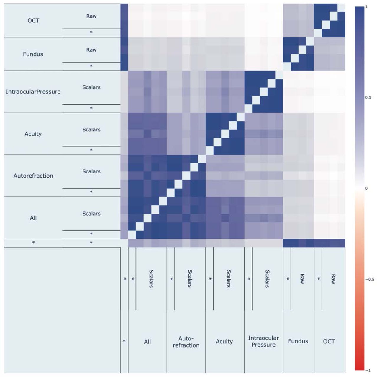
Fundus image-based and OCT image-based accelerated eye aging are genetically .299+-.025 correlated.
We compared fundus-based and OCT-based accelerated aging phenotypes in terms of their associations with non-genetic variables to understand if X-variables associated with accelerated aging in one eye dimension are also associated with accelerated aging in the other. For example, in terms of environmental variables, are the diets that protect against eye aging in terms of fundus image the same as the diets that protect against eye aging in terms of OCT image? We found that the correlation between accelerated brain anatomical and cognitive aging is .926 in terms of biomarkers, .704 in terms of associated clinical phenotypes, .830 in terms of diseases, .838 in terms of environmental variables and .748 in terms of socioeconomic variables (Figure 7). These results can be interactively explored at https://www.multidimensionality-of-aging.net/correlation_between_aging_dimensions/xwas_univariate.

Correlation between fundus-based and OCT-based accelerated eye aging in terms of associated biomarkers, clinical phenotypes, diseases, family history, environmental and socioeconomic variables
Discussion
We built the most accurate eye age predictor to date
By combining different eye phenotype datasets (fundus and OCT images, acuity, refractive error and intraocular pressure biomarkers) we built the most accurate eye age predictor to date, to the best of our knowledge. These datasets capture different facets of eye aging, as demonstrated by the limited phenotypic correlation of the accelerated eye aging definitions that we derived from them, and by the fact that combining them into an ensemble model improved our age prediction accuracy (R2) by 7% compared to the best performing model built on a single dataset (R2=83.6+-0.6% vs. 76.6+-1.3%).
Comparison between our models and the literature
A summary of the comparison between our models and the models reported in the literature can be found in Table S22. We are, to our knowledge, the first to predict age from optical coherence tomography images.
Eye fundus images
Chronological age was predicted on UKB using eye fundus images with a R2 value of 74±1% by Poplin et al. 5. We found that our ensemble model outperformed this prediction accuracy (R2=76.6±0.2%). One potential explanation for this difference is that Poplin et al.’s model was trained on only 48,000 UKB participants, whereas our model was trained on 90,000 participants. Poplin et al.’s model was however also trained on 236,000 EyePACS 14 images, so it is unclear if the sample size benefited their model or ours and/or from the different CNN architectures. For example, our InceptionV3 model slightly outperformed their model (R2=75.2±0.1%), whereas our InceptionResNetV2 model significantly underperformed (R2=69.1±0.2%).
More recently Nagasato et al. used transfer learning to train a VGG16 architecture on a far smaller sample size (n=85) using ultra-wide-field pseudo-color eye fundus images collected from participants aged 57.5±20.9 years to predict chronological age. However, they did not report their R-Squared value, only the slope of the regression coefficient between their predictor and chronological age (standard regression coefficient=0.833) 6.
Eye iris and corner images
Sgroi et al., Erbilek et al. and Rajput and Sable 7–9 predicted chronological age from iris images. Sgroi et al. trained a random forest on 630 scalar texture features extracted from 596 sample iris images to classify participants aged 22-25 years versus participants older than 35 years with an accuracy of 64%. Erbilek et al. built an ensemble of five simple geometric features extracted from the same iris images dataset. Using what they refer to as the sensitivity negotiation method, inspired by game theory, they obtained a classification accuracy of 75%. Rajput and Sable trained CNNs on 2,130 iris images collected from 213 participants aged 3-74 years and predicted chronological age with an MAE of 5-7 years 9.
Bobrov et al. trained CNNs on 8,414 eye corner images collected from participants aged 20-80 and predicted chronological age with a R2 value of 90.25% (estimated from the Pearson correlation) and a MAE of 2.3 years 10.
Features driving eye age prediction
The fact that eye age prediction is driven by spherical power and that the elastic net’s regression coefficient for this feature is positive is coherent with the fact that, with age, presbyopia becomes more prevalent 15. Presbyopia –also called age-related farsightedness– is a consequence of the loss of the ability for the eye to accommodate to focus on nearby objects and it corresponds to positive spherical power. Similarly, cylindrical power is a measure of astigmatism and increases with age 16–21, which explains its selection by the GBM and the positive regression coefficient in the elastic net.
Our attention maps highlighted the eye fundus vascular features, which is consistent with Poplin et al.’s attention maps 22. Ege et al. reported that with age, eye fundus images tend to become more yellow because of optimal imperfections in the refractive media 23, which was possibly leveraged by our neural networks and could explain why some non-vascularized regions were also highlighted. Finally, our attention maps highlighted most retinal layers in the OCT images. The diversity of the features highlighted by the different models is coherent with the fact that age-related changes occur in all ocular tissues 24.
Association of accelerated eye aging with genetic and non-genetic factors
The three GWAS we performed on the accelerated eye aging phenotypes highlighted variants in genes associated with the eye, such as HERC2 (associated with eye pigmentation), TTK (linked to retinoblastoma), RDH5 (involved in visual pigment synthesis and linked to fundus albipunctatus and fundus dystrophy), ABHD2 (linked to retinitis pigmentosa), PPL (present in keratinocytes), PDE6G (involved in the phototransduction signaling cascade of rod photoreceptors), TCF4 (involved in corneal dystrophy), ARMS2 (a component of the eye’s choroidal extracellular matrix, linked to age-related macular degeneration and retinal drusen), RP1L1 (a retinal-specific protein involved in photosensitivity and rod photoreceptors’ morphogenesis, and linked to Occult Macular Dystrophy and Retinitis Pigmentosa), and OCA2 (linked to iris pigmentation). These associations confirm the biological relevance of our predictor and suggest therapeutic targets to slow eye aging. Similarly, accelerated eye aging is associated with eyesight biomarkers, clinical phenotypes and diseases (e.g wearing glasses/contacts, presbyopia, cataract, retinal disorders, retinal detachments and breaks), further confirming its biological relevance.
Accelerated eye aging is also associated with biomarkers, phenotypes and diseases in other organ systems such as the cardiovascular system (e.g blood pressure, arterial stiffness, heart function, chest pain, hypertension, heart disease), metabolic health (e.g blood biochemistry, diabetes, obesity), brain health (e.g brain MRI biomarkers, mental health), the musculoskeletal system (e.g hand grip strength, heel bone densitometry, claudication, arthritis), mouth health, hearing, and others. Interestingly, accelerated eye aging is associated with facial aging. These associations suggest that the aging rate of the different organ systems is interconnected. It is for example well established that diabetes increases the risk of vision loss or blindness (diabetic retinopathy 25). Likewise, associations between cardiovascular and ocular health have been reported 26. More generally, we found that accelerated eye aging is associated with a poor general health (e.g overall health rating, personal history of disease and medical treatment). We explore the connection between eye aging and other organ systems’ aging in a different paper27.
In terms of environmental exposures, we found that general health factors such as getting poor sleep, smoking (including maternal smoking at birth) and lack of physical activity are associated with accelerated eye aging. Some diet variables such as cereal intake are associated with decelerated eye aging. Alcohol intake had a mixed association, with beer, cider and spirits being associated with accelerated eye aging, while usually taking alcohol with meals was associated with decelerated eye aging. We also found that playing video games and the time spent watching television were both associated with accelerated eye aging, which is coherent with the fact that screen time can strain the eye (computer vision syndrome) 28. Associations between sleep 29, smoking 30, physical activity 31, alcohol intake 32, diet 33 and ocular health have been reported in the literature, as well.
Participants with a higher socioeconomic status (e.g social support, income, education) were more likely to be decelerated eye agers, an effect likely due to an overall slower aging rate, itself mediated by better health literacy 34 and access to healthcare. For example, in the US, the richest 1% live approximately a decade older than their poorest 1% counterparts (10.1±0.2 years for females, 14.6±0.2 years longer for males) 35.
Limitations
To limit the need for computational resources, we extracted a 2D image from each 3D OCT image. Leveraging the full data with a three-dimensional convolutional neural network architecture would likely increase the age prediction accuracy.
The UK Biobank as a cross-sectional, observational dataset. As such, the correlations that we report in the XWAS do not allow us to infer causality.
A possible future direction would be to test if, on average, the right and left eyes age at significantly different rates.
Utility of eye age predictors
In conclusion, our eye age predictor can be used to monitor the eye aging process. The genetic and non-genetic associations we respectively report in the GWAS and the XWAS also suggest potential lifestyle and therapeutic interventions to slow or reverse eye aging. The GWAS in particular could shed light on the etiology of age-related eye disorders such as age-related macular degeneration 36. Finally, our eye age predictor could be used to evaluate the effectiveness of emerging rejuvenating therapies 37 on the eye. The DNA methylation clock is for example already used in clinical trials 38–40, but as aging is multidimensional 27, 41, multiple clocks might be needed to properly assess the effect of a rejuvenating therapeutic intervention on the different organ systems.
Methods
Data and materials availability
We used the UK Biobank (project ID: 52887). The code can be found at https://github.com/Deep-Learning-and-Aging. The results can be interactively and extensively explored at https://www.multidimensionality-of-aging.net/. We will make the biological age phenotypes available through UK Biobank upon publication. The GWAS results can be found at https://www.dropbox.com/s/59e9ojl3wu8qie9/Multidimensionality_of_aging-GWAS_results.zip?dl=0.
Software
Our code can be found at https://github.com/Deep-Learning-and-Aging. For the genetics analysis, we used the BOLT-LMM 42, 43 and BOLT-REML 44 softwares. We coded the parallel submission of the jobs in Bash 45.
Cohort Dataset: Participants of the UK Biobank
We leveraged the UK Biobank11 cohort (project ID: 52887). The UKB cohort consists of data originating from a large biobank collected from 502,211 de-identified participants in the United Kingdom that were aged between 37 years and 74 years at enrollment (starting in 2006). Out of these participants, approximately 87,000 had fundus and OCT images collected from them. The Harvard internal review board (IRB) deemed the research as non-human subjects research (IRB: IRB16-2145).
Data types and Preprocessing
The data preprocessing step is different for the different data modalities: demographic variables, scalar predictors and images. We define scalar predictors as predictors whose information can be encoded in a single number, such as eye spherical power, as opposed to data with a higher number of dimensions such as images (two dimensions, which are the height and the width of the image).
Demographic variables
First, we removed out the UKB samples for which age or sex was missing. For sex, we used the genetic sex when available, and the self-reported sex when genetic sex was not available. We computed age as the difference between the date when the participant attended the assessment center and the year and month of birth of the participant to estimate the participant’s age with greater precision. We one-hot encoded ethnicity.
Scalar biomarkers: acuity, autorefraction and intraocular pressure
We define scalar data as a variable that is encoded as a single number, such as eye spherical power or astigmatism angle, as opposed to data with a higher number of dimensions, such as images. The complete list of scalar biomarkers can be found in Table S4 under “Eye”. We did not preprocess the scalar data, aside from the normalization that is described under cross-validation further below.
Images
Eye fundus
The UKB contains eye fundus RGB images, with dimensions 1536*2048*3 pixels. Data from both the left eye (field 21015, 87,562 samples for 84,760 participants were collected) and the right eye (field 21016, 88,259 samples for 85,239 participants) was collected. We took the vertical symmetry of left eye images. We cropped the images to remove the black border surrounding the actual eye fundus images, which yielded centered square images with dimensions 1388*1388*3. Some of the images were low quality on visual inspection. For example, they had very low or very high luminosity. To reduce the prevalence of such images, we developed the following two-step heuristic. First, we computed the mode of the distribution for each of the three RGB layers. If the mode is strictly larger than 250 for both the red, the green and the blue channels, and has a frequency at least as high as 100,000 for the three channels, the image is removed. Second, we compute the median of the distribution for each of the three RGB channels. If the difference between the red median and the maximum between the green and blue medians is strictly smaller than ten, the image is removed. A sample of preprocessing OCT images can be found in Fig. S2.
Eyes optical coherence tomography
The UKB contains OCT 3D images from both the left eye (field 21017, 87,595 samples for 84,173 participants) and the right eye (field 21018, 88,282 images for 85,262 participants) (Fig. S3). Each sample contains 128 images of dimensions 650*512*1 grayscale pixels. We selected the image where the fovea pit is the deepest as the input for our models, as follows. First, for each sample, we discarded images before the 30th image and after the 105th image, because the fovea was never the deepest in the first or last images. Then we applied the fastNlMeansDenoising function from the openCV python library 46 to each of the remaining 75 images with the following hyperparameter values: h=30, templateWindowSize=7, searchWindowSize=7. We then applied OpenCV’s Canny edge algorithm 47 with 30 and 150 as the two thresholds for the hysteresis procedure to detect the surface of the retina. Instead of relying on a single threshold to detect edges, the hysteresis method consists in setting both an upper and lower threshold. Pixels whose gradient value is above the upper threshold are classified as belonging to an edge, and pixels whose gradient value is below the lower threshold are classified as non-edge. The remaining pixels, whose gradient value is between the two thresholds, are classified as an edge if they are connected to at least one edge pixel. For each column of pixels, we identified the surface of the retina as the first pixel encountered set to 1 by the canny edge algorithm, starting from the top of the image. We applied two smoothing methods (triangle moving average and Savitzky–Golay filter) to detect the surface (Fig. S4).
We then computed the curvature of the detected surface (Fig. S5), and we used the maximum curvature value for each of the 75 images. Next, we identified which of these 75 images had the maximal curvature, corresponding to the pit of the fovea. The list of maximal curvature for each image is a noisy function, so we applied the Savitzky–Golay filter to identify the image with the maximal curvature (Fig. S6). Finally, we cropped the selected image to center the fovea pit vertically to obtain the final images with dimension 500*512*3 pixels (Fig. S7). A sample of preprocessed OCT images can be found in Fig. S8.
To resolve prohibitory long training times, we resized the images so that the total number of pixels for each channel would be below 100,000.
Data augmentation
To prevent overfitting and increase our sample size during the training we used data augmentation 48 on the images. Each image was randomly shifted vertically and horizontally, as well as rotated. We chose the hyperparameters for these transformations’ distributions to represent the variations we observed between the images in the initial dataset. A summary of the hyperparameter values for the transformations’ distributions can be found in Table S24.
The data augmentation process is dynamically performed during the training. Augmented images are not generated in advance. Instead, each image is randomly augmented before being fed to the neural network for each epoch during the training.
Machine learning algorithms
For scalar datasets, we used elastic nets, gradient boosted machines [GBMs] and fully connected neural networks. For images we used two-dimensional convolutional neural networks.
Scalar data
We used three different algorithms to predict age from scalar data (non-dimensional variables, such as laboratory values). Elastic Nets [EN] (a regularized linear regression that represents a compromise between ridge regularization and LASSO regularization), Gradient Boosted Machines [GBM] (LightGBM implementation 49), and Neural Networks [NN]. The choice of these three algorithms represents a compromise between interpretability and performance. Linear regressions and their regularized forms (LASSO 50, ridge 51, elastic net 52) are highly interpretable using the regression coefficients but are poorly suited to leverage non-linear relationships or interactions between the features and therefore tend to underperform compared to the other algorithms. In contrast, neural networks 53, 54 are complex models, which are designed to capture non-linear relationships and interactions between the variables. However, tools to interpret them are limited 55 so they are closer to a “black box”. Tree-based methods such as random forests 56, gradient boosted machines 57 or XGBoost 58 represent a compromise between linear regressions and neural networks in terms of interpretability. They tend to perform similarly to neural networks when limited data is available, and the feature importances can still be used to identify which predictors played an important role in generating the predictions. However, unlike linear regression, feature importances are always non-negative values, so one cannot interpret whether a predictor is associated with older or younger age. We also performed preliminary analyses with other tree-based algorithms, such as random forests 56, vanilla gradient boosted machines 57 and XGBoost 58. We found that they performed similarly to LightGBM, so we only used this last algorithm as a representative for tree-based algorithms in our final calculations.
Images
Convolutional Neural Networks Architectures
We used transfer learning 59–61 to leverage two different convolutional neural networks 62 [CNN] architectures pre-trained on the ImageNet dataset 63–65 and made available through the python Keras library 66: InceptionV3 67 and InceptionResNetV2 68. We considered other architectures such as VGG16 69, VGG19 69 and EfficientNetB7 70, but found that they performed poorly and inconsistently on our datasets during our preliminary analysis and we therefore did not train them in the final pipeline. For each architecture, we removed the top layers initially used to predict the 1,000 different ImageNet images categories. We refer to this truncated model as the “base CNN architecture”.
We added to the base CNN architecture what we refer to as a “side neural network”. A side neural network is a single fully connected layer of 16 nodes, taking the sex and the ethnicity variables of the participant as input. The output of this small side neural network was concatenated to the output of the base CNN architecture described above. This architecture allowed the model to consider the features extracted by the base CNN architecture in the context of the sex and ethnicity variables. For example, the presence of the same anatomical feature can be interpreted by the algorithm differently for a male and for a female. We added several sequential fully connected dense layers after the concatenation of the outputs of the CNN architecture and the side neural architecture. The number and size of these layers were set as hyperparameters. We used ReLU 71 as the activation function for the dense layers we added, and we regularized them with a combination of weight decay 72, 73 and dropout 74, both of which were also set as hyperparameters. Finally, we added a dense layer with a single node and linear activation to predict age.
Compiler
The compiler uses gradient descent 75, 76 to train the model. We treated the gradient descent optimizer, the initial learning rate and the batch size as hyperparameters. We used mean squared error [MSE] as the loss function, root mean squared error [RMSE] as the metric and we clipped the norm of the gradient so that it could not be higher than 1.0 77.
We defined an epoch to be 32,768 images. If the training loss did not decrease for seven consecutive epochs, the learning rate was divided by two. This is theoretically redundant with the features of optimizers such as Adam, but we found that enforcing this manual decrease of the learning rate was sometimes beneficial. During training, after each image has been seen once by the model, the order of the images is shuffled. At the end of each epoch, if the validation performance improved, the model’s weights were saved.
We defined convergence as the absence of improvement on the validation loss for 15 consecutive epochs. This strategy is called early stopping 78 and is a form of regularization. We requested the GPUs on the supercomputer for ten hours. If a model did not converge within this time and improved its performance at least once during the ten hours period, another GPU was later requested to reiterate the training, starting from the model’s last best weights.
Training, tuning and predictions
We split the entire dataset into ten data folds. We then tuned the models built on scalar data and the models built on images using two different pipelines. For scalar data-based models, we performed a nested-cross validation. For images-based models, we manually tuned some of the hyperparameters before performing a simple cross-validation. We describe the splitting of the data into different folds and the tuning procedures in greater detail in the Supplementary.
Interpretability of the machine learning predictions
To interpret the models, we used the regression coefficients for the elastic nets, the feature importances for the GBMs, a permutation test for the fully connected neural networks, and attention maps (saliency and Grad-RAM) for the convolutional neural networks (Supplementary Methods).
Ensembling to improve prediction and define aging dimensions
We built a two-level hierarchy of ensemble models to improve prediction accuracies. At the lowest level, we combined the predictions from different algorithms on the same aging subdimension. For example, we combined the predictions generated by the elastic net, the gradient boosted machine and the neural network from the eye acuity scalar biomarkers. At the second level, we combined the predictions from the different eye dimensions into a general eye age prediction. The ensemble models from the lower levels are hierarchically used as components of the ensemble models of the higher models. For example, the ensemble model built by combining the algorithms trained on eye acuity variables is leveraged when building the general eye aging ensemble model.
We built each ensemble model separately on each of the ten data folds. For example, to build the ensemble model on the testing predictions of the data fold #1, we trained and tuned an elastic net on the validation predictions from the data fold #0 using a 10-folds inner cross-validation, as the validation predictions on fold #0 and the testing predictions on fold #1 are generated by the same model (see Methods - Training, tuning and predictions - Images - Scalar data - Nested cross-validation; Methods - Training, tuning and predictions - Images - Cross-validation). We used the same hyperparameters space and Bayesian hyperparameters optimization method as we did for the inner cross-validation we performed during the tuning of the non-ensemble models.
To summarize, the testing ensemble predictions are computed by concatenating the testing predictions generated by ten different elastic nets, each of which was trained and tuned using a 10-folds inner cross-validation on one validation data fold (10% of the full dataset) and tested on one testing fold. This is different from the inner-cross validation performed when training the non-ensemble models, which was performed on the “training+validation” data folds, so on 9 data folds (90% of the dataset).
Evaluating the performance of models
We evaluated the performance of the models using two different metrics: R-Squared [R2] and root mean squared error [RMSE]. We computed a confidence interval on the performance metrics in two different ways. First, we computed the standard deviation between the different data folds. The test predictions on each of the ten data folds are generated by ten different models, so this measure of standard deviation captures both model variability and the variability in prediction accuracy between samples. Second, we computed the standard deviation by bootstrapping the computation of the performance metrics 1,000 times. This second measure of variation does not capture model variability but evaluates the variance in the prediction accuracy between samples.
Eye age definition
We defined the eye age of participants for a specific eye dimension as the prediction outputted by the model trained on the corresponding dataset, after correcting for the bias in the residuals.
We indeed observed a bias in the residuals. For each model, participants on the older end of the chronological age distribution tend to be predicted younger than they are. Symmetrically, participants on the younger end of the chronological age distribution tend to be predicted older than they are. This bias does not seem to be biologically driven. Rather it seems to be statistically driven, as the same 60-year-old individual will tend to be predicted younger in a cohort with an age range of 60-80 years, and to be predicted older in a cohort with an age range of 60-80. We ran a linear regression on the residuals as a function of age for each model and used it to correct each prediction for this statistical bias.
After defining biological age as the corrected prediction, we defined accelerated aging as the corrected residuals. For example, a 60-year-old whose eye fundus images predicted an age of 70 years old after correction for the bias in the residuals is estimated to have an eye age of 70 years, and an accelerated eye aging of ten years.
It is important to understand that this step of correction of the predictions and the residuals takes place after the evaluation of the performance of the models but precedes the analysis of the eye ages properties.
Genome-wide association of accelerated eye aging
The UKB contains genome-wide genetic data for 488,251 of the 502,492 participants79 under the hg19/GRCh37 build.
We used the average accelerated aging value over the different samples collected over time (see Supplementary - Generating average predictions for each participant). Next, we performed genome wide association studies [GWASs] to identify single-nucleotide polymorphisms [SNPs] associated with accelerated aging in each eye dimension using BOLT-LMM 42, 43 and estimated the the SNP-based heritability for each of our biological age phenotypes, and we computed the genetic pairwise correlations between dimensions using BOLT-REML 44. We used the v3 imputed genetic data to increase the power of the GWAS, and we corrected all of them for the following covariates: age, sex, ethnicity, the assessment center that the participant attended when their DNA was collected, and the 20 genetic principal components precomputed by the UKB. We used the linkage disequilibrium [LD] scores from the 1,000 Human Genomes Project1. 80. To avoid population stratification, we performed our GWAS on individuals with White ethnicity.
Identification of SNPs associated with accelerated eye aging
We identified the SNPs associated with accelerated eye aging dimensions using the BOLT-LMM 42, 43 software (p-value of 5e-8). The sample size for the genotyping of the X chromosome is one thousand samples smaller than for the autosomal chromosomes. We therefore performed two GWASs for each aging dimension. (1) excluding the X chromosome, to leverage the full autosomal sample size when identifying the SNPs on the autosome. (2) including the X chromosome, to identify the SNPs on this sex chromosome. We then concatenated the results from the two GWASs to cover the entire genome, at the exception of the Y chromosome.
We plotted the results using a Manhattan plot and a volcano plot. We used the bioinfokit 81 python package to generate the Manhattan plots. We generated quantile-quantile plots [Q-Q plots] to estimate the p-value inflation as well.
Heritability and genetic correlation
We estimated the heritability of the accelerated aging dimensions using the BOLT-REML 44 software. We included the X chromosome in the analysis and corrected for the same covariates as we did for the GWAS. Using the same software and parameters, we computed the genetic correlations between accelerated aging in the two image-based eye dimensions.
We annotated the significant SNPs with their matching genes using the following four steps pipeline. (1) We annotated the SNPs based on the rs number using SNPnexus 82–86. When the SNP was between two genes, we annotated it with the nearest gene. (2) We used SNPnexus to annotate the SNPs that did not match during the first step, this time using their genomic coordinates. After these two first steps, 30 out of the 9,697 significant SNPs did not find a match. (3) We annotated these SNPs using LocusZoom 87. Unlike SNPnexus, LocusZoom does not provide the gene types, so we filled this information with GeneCards 12. After this third step, four genes were not matched. (4) We used RCSB Protein Data Bank 88 to annotate three of the four missing genes.
Non-genetic correlates of accelerated eye aging
We identified non-genetically measured (i.e factors not measured on a GWAS array) correlates of each aging dimension, which we classified in six categories: biomarkers, clinical phenotypes, diseases, family history, environmental, and socioeconomic variables. We refer to the union of these association analyses as an X-Wide Association Study [XWAS]. (1) We define as biomarkers the scalar variables measured on the participant, which we initially leveraged to predict age (e.g. blood pressure, Table S4). (2) We define clinical phenotypes as other biological factors not directly measured on the participant, but instead collected by the questionnaire, and which we did not use to predict chronological age. For example, one of the clinical phenotypes categories is eyesight, which contains variables such as “wears glasses or contact lenses”, which is different from the direct refractive error measurements performed on the participants, which are considered “biomarkers” (Table S7). (3) Diseases include the different medical diagnoses categories listed by UKB (Table S10). (4) Family history variables include illnesses of family members (Table S13). (5) Environmental variables include alcohol, diet, electronic devices, medication, sun exposure, early life factors, medication, sun exposure, sleep, smoking, and physical activity variables collected from the questionnaire (Table S16). (6) Socioeconomic variables include education, employment, household, social support and other sociodemographics (Table S19). We provide information about the preprocessing of the XWAS in the Supplementary Methods.
Author Contributions
Alan Le Goallec: (1) Designed the project. (2) Supervised the project. (3) Predicted chronological age from images. (4) Computed the attention maps for the images. (5) Ensembled the models, evaluated their performance, computed biological ages and estimated the correlation structure between the eye aging dimensions. (6) Performed the genome wide association studies. (5) Designed the website. (6) Wrote the manuscript.
Samuel Diai: (1) Predicted chronological age from scalar features. (2) Coded the algorithm to obtain balanced data folds across the different datasets. (3) Wrote the python class to build an ensemble model using a cross-validated elastic net. (4) Performed the X-wide association study.(5) Implemented a first version of the website https://www.multidimensionality-of-aging.net/.
Sasha Collin: (1) Preprocessed the OCT images. (2) Preprocessed the fundus images.
Théo Vincent: (1) Website data engineer. (2) Implemented a second version of the website https://www.multidimensionality-of-aging.net/.
Chirag J. Patel: (1) Supervised the project. (2) Edited the manuscript. (3) Provided funding.
Data Availability
We used the UK Biobank (project ID: 52887). The code can be found at https://github.com/Deep-Learning-and-Aging. The results can be interactively and extensively explored at https://www.multidimensionality-of-aging.net/. We will make the biological age phenotypes available through UK Biobank upon publication. The GWAS results can be found at https://www.dropbox.com/s/59e9ojl3wu8qie9/Multidimensionality_of_aging-GWAS_results.zip?dl=0.
https://github.com/Deep-Learning-and-Aging
https://www.multidimensionality-of-aging.net/
https://www.dropbox.com/s/59e9ojl3wu8qie9/Multidimensionality_of_aging-GWAS_results.zip?dl=0
Conflicts of Interest
None.
Funding
NIEHS R00 ES023504
NIEHS R21 ES25052.
NIAID R01 AI127250
NSF 163870
MassCATS, Massachusetts Life Science Center Sanofi
The funders had no role in the study design or drafting of the manuscript(s).
Acknowledgments
We would like to thank Raffaele Potami from Harvard Medical School research computing group for helping us utilize O2’s computing resources. We thank HMS RC for computing support. We also want to acknowledge UK Biobank for providing us with access to the data they collected. The UK Biobank project number is 52887.
Footnotes
↵+ Co-second authors
References
- 1.↵
- 2.↵
- 3.↵
- 4.↵
- 5.↵
- 6.↵
- 7.↵
- 8.
- 9.↵
- 10.↵
- 11.↵
- 12.↵
- 13.↵
- 14.↵
- 15.↵
- 16.↵
- 17.
- 18.
- 19.
- 20.
- 21.↵
- 22.↵
- 23.↵
- 24.↵
- 25.↵
- 26.↵
- 27.↵
- 28.↵
- 29.↵
- 30.↵
- 31.↵
- 32.↵
- 33.↵
- 34.↵
- 35.↵
- 36.↵
- 37.↵
- 38.↵
- 39.
- 40.↵
- 41.↵
- 42.↵
- 43.↵
- 44.↵
- 45.↵
- 46.↵
- 47.↵
- 48.↵
- 49.↵
- 50.↵
- 51.↵
- 52.↵
- 53.↵
- 54.↵
- 55.↵
- 56.↵
- 57.↵
- 58.↵
- 59.↵
- 60.
- 61.↵
- 62.↵
- 63.↵
- 64.
- 65.↵
- 66.↵
- 67.↵
- 68.↵
- 69.↵
- 70.↵
- 71.↵
- 72.↵
- 73.↵
- 74.↵
- 75.↵
- 76.↵
- 77.↵
- 78.↵
- 79.↵
- 80.↵
- 81.↵
- 82.↵
- 83.
- 84.
- 85.
- 86.↵
- 87.↵
- 88.↵


