
Abstract
We devise a significance test for covariance of samples not drawn independently, but with known inter-sample covariance structure. The test distribution we propose is a linear combination of χ2 distributions, with positive and negative coefficients. The corresponding cumulative distribution function can be efficiently calculated with Davies algorithm at high precision. As an application, we propose a test for dependence between SNP-wise effect sizes of two genome-wide association studies at the level of genes. The test can be extended to detect gene-wise causal links. We illustrate this method by uncovering potential shared genetic links between severity of Covid-19, taking of class M05B medication (drugs affecting bone structure and mineralization), Vitamin D (25OHD) and Calcium concentrations. In particular, our method detects a potential role played by chemokine receptor genes linked to TH1 versus TH2 immune reaction, a gene related to integrin beta-1 cell surface expression, and other genes potentially impacting severity of Covid-19.
I. INTRODUCTION
Pearson’s sample correlation is one of the most used techniques in data analysis, independent of the specific field of science. It is defined as the covariance divided by the standard deviations of two random variables and gives a measure of linear dependence. The core underlying requirement is that the observed samples are drawn independently from a joint bivariate distribution. However, not all applications possess independently drawn samples.
One particular application with dependent samples can be found in genome-wide association studies (GWAS). In detail, GWAS correlate genomic single nucleotide polymorphisms (SNPs) with phenotypes in a study population, usually independently SNP by SNP. By now, thousands of such GWAS have been conducted and identified a plethora of statistically significant SNPs associated with disease risks and other relevant phenotypes, consistent with a polygenic genetic architecture [1]. These studies yield valuable information to better understand complex diseases and aid drug discovery and re-purposing.
However, due to Linkage Disequilibrium (LD) (cf., [2]), many SNPs in close proximity are not independent, and this leads to dependencies between observed SNP effect sizes. This is of particular relevance in the aggregation to gene and pathway effect sizes. In this context, a pathway is understood as a functional set of genes and the SNP effect sizes in the gene regions are aggregated to a single effect. If not corrected for LD, the resulting gene and pathway scores may reflect the level of importance for the phenotype inaccurately. For this reason, techniques and tools have been developed to correct for LD in the aggregation process, like for example PASCAL [3] and MAGMA [4]. These tools mainly differ in how they map SNP effect sizes to genes, how the LD structure is accounted for, and details of the numerical procedure to estimate significance.
Often, a SNP is significant for more than one trait, i.e., two or more traits may share the same genetic origin (pleiotropy) [5]. In particular, such a shared genetic component hints at that the same functional pathology may contribute to several diseases, cf., [6]. At the gene level, usually a gene is considered to be relevant for two different traits if the gene carries a significant SNP effect size in both traits. However, this may not be a good criterion under all circumstances. Protein coding genes often contain several independent LD blocks. Therefore, two traits may associate with genetic variation in two or more functionally different blocks of SNPs within the same gene, which may independently be significant. Hence, even though the two traits share the same significant gene, they may not share the same functional genetic mechanism. In order to call pleiotropy of a gene, one should therefore move beyond comparing single variants, and take all SNPs in the gene region into account. For a classic review on pleiotropy in complex traits we refer to [5]. In the following, some of the more novel methods proposed in the literature to uncover a fine-coarse shared genetic origin of two traits from GWAS summary statistics will be discussed.
One early method is the Bayesian based test of colocalisation between GWAS pairs of [7]. This method assumes that at most one association is present for each trait in the region of interest. The extension to the general case for the usually available single SNP summary statistics appears, however, to be more involved.
A more recent method which attracted widespread attention and adoption to study the genetic component and correlation between traits is LD score regression [8, 9]. In this Ansatz, the effect sizes are considered as random variables and thereby naturally define a notation of heritability and (linear) genetic correlation. In particular, this leads to a simple and computational efficient method to calculate the correlation coefficient via regression. However, stratifying LD score regression onto the level of genes is in general difficult. Mainly because SNPs in the same genomic region are often in high LD, as already mentioned above. Hence, the variables entering the linear correlation may be highly dependent, and this has to be corrected for. Similarly, the standard errors and p-values are estimated via resampling (jackknife). But this demands independent samples, which is not the case for strong LD.
Another method to estimate local genetic covariance and correlation has been introduced in [10]. However, this method requires the computation of the inverse SNP-SNP correlation matrix, which is in general problematic as it often would need regularization.
Here, we instead put forward to simply consider the raw second cross moment between the overlapping SNPs of two traits in a gene region, corrected for LD, to call pleiotropy. This gives us a simple, but systematic definition of co-significance of a gene for two traits, i.e., if the SNP-wise cross-moment is significant. For a single overlapping SNP this reduces to testing against the product-normal distribution, and hence corresponds to a multiplicative meta-analysis, rather than an additive one like Fisher’s. Though our Ansatz does not intrinsically disentangle genetic and potential additional joint residual contributions, it nevertheless has utility in uncovering genes of relevance to more than one trait, as we will illustrate with an explicit example of current high interest in this work.
The technical novelty of the method we present here, which allows to perform such a significant test of covariance in the case of dependent samples, is the observation that one can express the underlying test distribution in terms of a linear combination of χ2 distributions, with a mixture of positive and negative coefficients. This allows one to take systematically into account not only isolated significant SNPs for calling a gene co-significant for two traits, but all common SNPs in the gene region. The assumption we have to make is that there is an underlying joint normal distribution, and the dependency pattern of the SNPs is known (for instance, the pattern can be approximated from a reference population). Furthermore, we assume that the study populations of the two traits do not have overlapping samples and that both populations can be approximated by an identical reference panel.
In the spirit of Mendelian randomization, the test can be extended to test for a possible causal relation between the two traits, mediated by the tested gene. However, possible confounders have to be excluded by other means.
The outline of this paper is as follows.
In sections II and III we will introduce the probability distributions of relevance for this work. Most readers are probably familiar with the χ2 distribution reviewed in section II. The role played in this work by the χ2 is essential, as all the other distributions we consider can be expressed as a linear combination of χ2 distributions. This holds in particular for the product-normal distribution, as we will see in section III, as well as for the Variance-Gamma distribution discussed in appendix B. The core sections of this paper constitute IV, in which we explain how we can perform a significance test of independence under the conditions described above, and section V, in which we derive a way to calculate the cumulative distribution function of a particular ratio distribution of relevance for a causality test. Simulated examples are discussed in section VI, followed by an application to real GWAS data in section VII. As illustrative example, we will use the developed technique to find computational predictions for shared genetic links between severity of Covid-19, class M05B medication taking, and Vitamin D and Calcium concentrations. In particular, we detect a potential role for severity of Covid-19 played by chemokine receptor genes linked to TH 1 versus TH 2 immune reaction, and a gene related to integrin beta-1 cell surface expression. Several other genes related to Covid-19, discussed before elsewhere in the literature, are replicated. In addition we uncover hints for a potential protective and/or therapeutic pathway related to taking of specific immune related medications (H03A, L04 and M01A).
II. LINEAR COMBINATION OF χ2DISTRIBUTIONS
Let us denote as  the χ2-distribution with n degrees of freedom. It is well known that the sum of N independent
  distributed random variables zi is again χ2 distributed, i.e.,
 However, no closed analytic expression for the distribution Ξ of a general linear combination,
 with ai some real coefficients, is known. Nevertheless, a variety of numerical algorithms exist to compute the cumulative distribution function (cdf) of Ξ, denoted as FΞ, exactly up to a desired precision. Perhaps most well known are variants of Ruben’s algorithm [11–13] and Davies algorithm [14]. The latter of which is of most relevance for this work, as it allows for negative ai.
With FΞ at hand, for given real x a right tail probability p (p-value), can be calculated as
 One should note that the achievable precision of p calculated via (2) is limited by the available machine precision.
Note that also a varity of approximations to the distribution Ξ exists, cf., [15]. One of the more well known methods is the Satterthwaite-Welch approximation [16, 17], which matches the first two moments of Ξ to a Gamma distribution, denoted as Γ. In detail [18],
 with
with
 Here, di denotes the ith degree-of-freedom parameter of the ith χ2 in equation (1) and i ∈ {1, …, N}.
To our knowledge, the quality of second order approximations to Ξ at very high precision (below double precision) has not been evaluated in the literature, cf., [15].
III. PRODUCT-NORMAL DISTRIBUTION
A central role in this work is played by the product-normal distribution, the distribution of the product of two normal distributed random-variables w and z. The moment generating function for joint normal samples with correlation ϱ reads [19]
 The core observation we will make use of is that the above moment generating function factorizes into moment generating functions of the gamma distribution,
 , i.e.,
 Therefore,
 For general parameters of the two gamma distributions the corresponding difference distribution is known as the bilateral gamma distribution [20]. One should note that the subtraction is in the distributional sense. Hence, even for ϱ = 0, the difference does not vanish.
Due to the well known relation between the gamma and χ2 distributions, one can also express the product-normal distribution in terms of the χ2 distribution introduced in the previous section. In detail,
 The cdf of the product-normal can therefore be efficiently calculated using Davies algorithm, as the distribution (5) is simply a linear combination of
  distributions. A similar relation can be derived for the product distribution of non-standardized Gaussian variables, albeit in terms of the non-central χ2 distribution, cf., appendix A. Note that the relation (4) allows for a simple analytic derivation of a closed form solution for the product-normal pdf, but not for the cdf. For completeness, details can be found in appendix B.
We conclude that the cdf of the product normal distribution can be calculated with Davies algorithm. In particular, note that for ϱ = 0 we can not make use of the Satterthwaite-Welch approximation to calculate the cdf, as the first cumulant vanishes and therefore (3) is not well defined.
IV. COVARIANCE SIGNIFICANCE TEST
Consider the index
 with wi and zi N independent samples of two random variables z, w ~ 𝒩 (0, 1). The index can also be written as
 with 𝔼 denoting the expectation. Clearly, I is proportional to the standard empirical covariance of w and z.
For independent pairs of samples, the sampling distribution of I is simply a sum of independent product-normal distributions, hence we infer from the previous sections that for identically correlated random variables
 In particular, for ϱ = 0, we have that I ~ X(N, 1), with X being the Variance-Gamma distribution discussed in more detail in appendix B. As mentioned already before, one should note that the difference is in the distributional sense and therefore generally non-vanishing. A null assumption of zero correlation (or some other fixed value) can therefore be tested via (2), as the cdf for I can be calculated explicitly and efficiently with Davies algorithm.
We have now all ingredients in place to discuss the problem we want to address with this paper. The main advantage of the above significance test is that it is straight-forward to relax the requirement of sample independence. That is, we can view the index I as a scalar product of random samples of w ~ 𝒩 (0, Σw) and z ~ 𝒩 (0, Σz), with 𝒩 denoting here the multivariate Gaussian distribution and Σ. covariance matrices. For Σ. = 1, the corresponding distribution of I is given by (7). In the general case, the inter-dependencies can be corrected for as follows.
We make use of the eigenvalue decompositions  and
and  , with Λ the diagonal matrix of eigenvalues of Σ., to decorrelate the elements of each set. The index I can then be written as
 with ŵ ~ 𝒩 (0, Λw),
  and
and  In components, I reads
 The case of interest for this paper is Σw = Σz =: Σ such that K is the identity matrix. In this case, making use of the moment generating function of the product-normal, as in section III, we can show that under the null of w and z being independent
 with λi the ith eigenvalue of Σ. Hence, I is distributed according to a linear combination of
  distributions with positive and negative coefficients, and therefore the cdf and tail probability can be calculated with Davies algorithm.
Note that the above discussion can be extended to non-standardized variables (for ϱ = 0) via making use of the result of appendix A.
V. RATIO SIGNIFICANCE
Consider the normalized index
 with w and z as in the previous section, in particular independent. The cdf for R can be calculated as follows (similarly for w and z interchanged). Clearly, for Σw = Σz = Σ we have that
 We define
  such that
  . Note that the component-wise correlation coefficient ϱ between
  and
and  reads
reads
 Hence, from (5) and (A1) we deduce that
 We conclude that
 Hence, the cdf of the ratio (9) can be as well calculated with Davies algorithm. A consistency check can be performed as follows. In one-dimension, we have that R has to be Cauchy distributed. The corresponding cdf is given by
  . Evaluation for various r shows agreement with values calculated from (10) in the one-dimensional case. Note that for non-standardized wi and zi similar expressions can be derived, albeit in terms of the non-central χ2 distribution, cf., appendix A.
VI. EXAMPLE 1: SIMULATIONS
In the following, several examples will be discussed, illustrating more specific aspects and applications of the theoretical material presented so far.
A. Single element
It is interesting to discuss the single element case in more detail. The distribution (8) simplifies for N = 1 to
 which corresponds to the uncorrelated product normal distribution, cf., (5). One should interpret the index I for N = 1 as a measure of coherence (or anti-coherence) between z and w. The significance threshold curve for a fixed desired p-value, say pI = 10−8, is illustrated in figure 1. One should note that the curve is unbounded. That is, for given w, there is always a corresponding z such that the resulting product I is significant. For instance, this differs from Fisher’s exact method to combine p-values (meta-analysis). Fisher’s method combines two p-values pi
  . Due to its additive nature, Fisher’s method results in a bounded significance curve. In the extreme case of one of the p-values being equal to one, the significance simply corresponds to the other p-value. In contrast, for the product-normal divergence between the p-values is penalized. If one of the p-values is large, the other one has to be exponentially smaller in order to stay on the same significance curve, cf., figure 1. Therefore, one should see Fisher’s method as being additive in the evidence, while the product-normal based method as being multiplicative.

Significance threshold curves of I (blue line) and R (green line) in the one element case for pI = 10−8, respectively, pR = 10−1, in the positive domain. The orange dotted lines mark the symmetric point with pz = pw ~ 5 × 10⁻⁵. The red dotted lines mark pw = 0.05 and pz ~ 10−16. The gray dashed line illustrates the significance threshold based on Fisher’s method with pF = 10−8.
The linear threshold curve of R for pR = 10−1, defined in (9), is also shown in figure 1. Note the small slope, even for rather large p-values.
B. Two elements
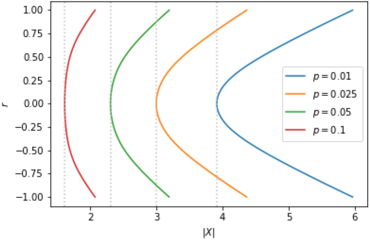
The importance of correcting for the inter-dependence between the elements of w and z can be seen easily in the N = 2 case. Consider the covariance matrices,
 such that w ~ 𝒩 (0, Σ) and z ~ 𝒩 (0, Σ), and with r varying. In figure 2 we show various significance threshold curves of I for varying r, as calculated from the distribution (8). Clearly, for increasing inter-element correlation, the significance threshold level rises. The magnitude of the effect increases with the desired level of significance.

Significance threshold curves of I in the two element case under variation of the inter-element correlation (y-axis). The x-axis corresponds to the argument of the tail probability defined in equation (2). The gray dotted lines mark the minimal value obtained for zero correlation.
C. Normal draws
Consider a correlation matrix Σ of dimension one hundred with off-diagonal elements identically set to 0.2. We draw 1000 pairs of independent samples of 𝒩 (0, Σ) and calculate for each pair I defined in (6). A p-value is then obtained for each index value for the linear combination of χ2 distributions (8) (also referred to as weighted χ2), and for the gamma-variance distribution (B4). Recall that the latter does not correct for the off-diagonal correlations. We repeat the experiment with the off-diagonal elements set to 0.8, resulting in a stronger element-wise correlation. Resulting QQ-plots for both cases are shown in figure 3.
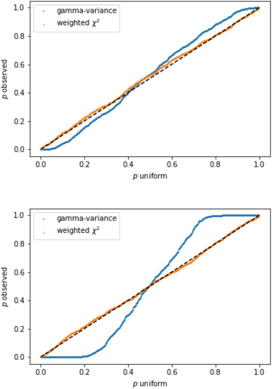
QQ-plots of observed p-values resulting from the index I for 1000 pairs of samples of 𝒩 (0, Σ) against uniform p-values. Top: Off-diagonal elements of Σ set to 0.2. Bottom: Off-diagonal set to 0.8. The blue curve is obtained using the gamma-variance distribution to perform the statistical test, while the orange curve is obtained via the weighted χ2 distribution. The latter corrects for the correlation and therefore is well calibrated.
We observe that the gamma-variance distribution (7) (with ϱ = 0) indeed becomes unsuitable for increasing element-wise correlation of the data sample elements. In detail, not correcting for the inter-sample correlation leads to more and more false positives with increasing correlation strength. In contrast, the weighted χ2 distribution (8) yields stable results in both the weakly and strongly correlated regime, as is evident in figure 3.
VII. EXAMPLE 2: GENETIC COHERENCE
A. Generalities
As explained in the introduction, a prime example of very strong inter-element correlations are SNPs in LD.
Recall that the univariate least squares estimates of the effect sizes β reads
 with xi the ith column of the genotype matrix X of dimension (n, p) and y the phenotype vector of dimension n.Both x and y are mean centered and standardized. n is the number of samples and p the number of SNPs. The central limit theorem and standardization ensures that for n sufficiently large
  .
.
As a multi-variate model, we have
 with α the vector of p true effect sizes and ϵ the n-dimensional vector of residuals with components assumed to be ϵi ~ 𝒩 (0, 1) and independent. Substituting the multi-variate model into (11), yields
a. Fixed effect size model
Under the null assumption that α = 0 (no effects), we infer that
 We can stack an arbitrary collection of such zi to a vector z via stacking the xi to a matrix x, such that
 with
with  . Note that we made use of the affine transformation property of the multi-variate normal distribution.
It is important to be aware that z is only a component-wise univariate estimation, and hence the null model (12) is for a collection of SNPs with effect sizes estimated via independent regressions.
b. Effect sizes as random variables
We can also take the effects to be random variables themselves. Let us assume that independently αi ~ 𝒩 (0, h2/p), with h referred to as heritability. We then have that
 such that
 with
with  , and where we assumed that α and ϵ are independent. Two remarks are in order. As X runs over all SNPs, calculation of L usually requires an approximation, for instance, via a cutoff. Furthermore, the null model (13) requires an estimate of the heritability. Such an estimate can be obtained for via LD score regression [9].
c. Genetic coherence
For this paper, it is only of importance that in both cases a. and b., the null model for z is a multi-variate Gaussian.
Therefore,
 with λi the ith eigenvalue of the covariance matrix of the Gaussian. As discussed in detail in [3], a GWAS gene enrichment test can be performed via testing against (14). This effectively tests against the expected variance of SNPs significances in the gene.
What we propose here, is to use (8) of section IV, i.e.,
 for w and z resulting from two different GWAS phenotypes, to test for co-significance of a gene for two GWAS. In more detail, a significance test can be performed either against the right tail of the null distribution (15) (coherence), or against the left tail (anti-coherence).
A clarifying remark is in order. Note that we do not centralize w and z over the gene SNPs. Hence, we do not test for covariance, but for a non-vanishing second cross-moment. After de-correlation, it is best to interpret this as testing independently each joint SNP in the gene for a coherent deviation from the null expectation. Therefore we refer to this test as testing for genetic coherence, or simply as cross-scoring. An example will be discussed below. For simplicity, in this work we only consider the fixed effect size model a. and assume that the correlation matrix Σ obtained from an external reference panel is a good approximation for both GWAS populations.
d. Direction of association
The direction of effect of the aggregated gene SNPs can be estimated via the index
 In detail, making use of the Cholesky decomposition Σ = CCT (requires regularization of the estimated Σ), and the affine transform property of the multi-variate Gaussian, we have that as null
 with |.|F the Frobenius norm. Testing for deviations from D in the right or left tail, gives an indication of the direction of the aggregated effect size. Note that the (anti)-coherence test between pairs of GWAS introduced above is alone not sufficient to determine the direction for a GWAS pair, but requires in addition to test at least one GWAS via (16) to determine the base direction of the aggregated gene effect. Furthermore, at least one GWAS needs to carry sufficiently oriented signal in the gene such that (16) can succeed. We will also refer to testing for deviations from (17) as D-test.
e. Ratio test
Note that the ratio
 with
with  and
and  i.i.d. 𝒩 (0, 1), and λi the ith eigenvalue of Σ, can be interpreted as the weighted least squares solution in the case of heteroscedasticity for the regression coefficient of the linear regression between the de-correlated effect sizes of the two GWAS. Therefore, with the cdf for R derived in section V, we can test for a significant deviation from the null expectation of no relation. Note that in general R is not invariant under interchange of response and explanatory variable, and may be used under certain conditions to make inference about the causal direction, cf., multi-instrument Mendelian randomization, in particular [21]. The main idea can be readily sketched.
Note first that the ratio test tries to detect genes that are maximal (anti)-coherent over the SNP effects between two GWAS, but at the same time carry minimal variance in one of the GWAS, as is clear from (18). The purpose of this, at first sight somewhat non-intuitive, statistical test becomes more clear if one thinks in terms of one GWAS trait as being the exposure and the other as outcome. If the ratio tested gene does carry minimal SNP variance only over the outcome, but on the same time SNP coherence between the exposure and outcome, the causal direction from exposure to outcome is implied, if the exposure is confirmed to be associated to the gene via pV obtainable from (14), and confounding factors can be excluded. The setup is illustrated in figure 4.

Interpretation of the ratio test. The test detects potential gene-wise causal relations between a GWAS trait viewed as exposure (E) and a GWAS trait viewed as outcome (O). The association of the exposure has to be confirmed independently via (14). Potential confounders (C) have to be excluded by other means.
B. Single SNP
As we have seen in section VI, the product normal combines evidence in a multiplicative way. Obtaining a combined single SNP p-value from two different GWAS in this way comes however with a potential pitfall. Namely,if one of the SNPs p-values is small enough, we can always achieve co-significance. We see two possible strategies to mitigate this.
One way would be to introduce a hard cutoff for very small SNP-wise p-values. The precise cutoff depends on the desired co-significance to achieve, and the amount of possible uplift of large p-values one finds acceptable. The dynamics is clear from figure 1. If we target a co-significance of p = 10−8 and accept to consider SNPs with a p-value of 0.05 or less in one GWAS to be sufficiently significant, we have to cutoff p-values around 10−16, cf., the red dotted lines in the figure. While such a cutoff ensures that no SNPs with p-values above in one GWAS can become co-significant due to very high significance (i.e. p-value below 10−16) in the other GWAS, applying such a hard cutoff point hampers distinguishing differences in co-significances.
Another possibility would be to first uniformize the p-values via ranking. That is, the p-values for all shared SNPs between the two GWAS are sorted for each GWAS and new p-values are calculated from the ranks. These ranked p-values (often also referred to as QQ-normalized) are then used as input for (15), after an appropriate inverse transform. Note that an unintended uplift of p-values, say above 0.05, could happen in the ranked case only for more than 1016 joined SNPs (i.e., much more than in any realistic case).
Since the ranking allows one to consider two GWAS with significantly different signal strength without the need to introduce an adhoc cutoff, the QQ-normalization is our approach of choice, and will be utilized in the following example. Note that also for the ratio test QQ-normalization is preferred in order to compensate for different signal strength between the GWAS.
C. Application to Covid-19 GWAS
1. Coherence test
We consider the meta-GWAS summary statistics on very severe respiratory confirmed Covid-19 cases versus the general population of European ancestry and without UK Biobank data contribution [22] (A2 ALL eur leave ukbb 23andme, release 7. Jan. 2021). This GWAS shows significant gene enrichment on chromosomes 3 and 12, as can be inferred via testing against the null model (14) with fixed effect sizes. The Manhattan plot for the resulting gene p-values on these chromosomes is shown in figure 5. Note that even though the GWAS analysis implicates a set of disease relevant genes, the key causal drivers have not yet been identified.

Manhattan plot showing the strong gene enrichment on chromosomes 3 and 12 for the severe Covid-19 GWAS. The Bonferroni significance threshold is taken to be 2.67 × 10⁻⁶ (0.05 divided by number of tested genes, red dotted line). Only a selection of significant genes are labeled.
We cross-scored this GWAS against a panel of GWAS on medication within the UK Biobank [23]. These GWAS on medication take intake of 23 common types of medications as traits. Hence, in cross-scoring against the severe Covid-19 GWAS we hope to uncover whether there is a shared genetic architecture between severity and pre-disposition to taking specific medications. Note that we minimized possible effects of sample overlap via restricting to the Covid-19 meta-GWAS without UK Biobank contribution.
All calculations have been performed with the python package PascalX [24] with default settings, using the European subpopulation of the 1000 Genome Project [25] as reference panel to estimate the SNP-SNP correlations Σ. Only protein coding genes have been considered and the gene window has been extended by 50k at the transcription start and end position. The cross-scoring has been performed over the extended window. For the reason discussed in section VII B, we uniformize the raw GWAS p-values via joint rank transform. Note that we use the signs from the direction of association (β).
a. Coherence
The cross-scoring results for the coherence test are shown in figure 6. The medication group M05B (drugs affecting bone structure and mineralization) shows enrichment in very severe Covid-19. We show the Manhattan plot resulting from the null model (12) and the index (15) for the medication group M05B in figure 7. We observe that genes in the well-known Covid-19 peak locus on chromosome 3 appear to be coherent with M05B medication taking, with the strongest significance for the chemokine receptor genes CCR1, CCR3 and LZTFL1 in the region chr3p21. We test the orientation of the aggregated associations of these genes via (16) over the Covid-19 GWAS and find a positive direction (right tail).

Resulting p-values for cross scoring 23 drug classes GWAS against very severe Covid-19 GWAS for coherence, respectively, anti-coherence. Each data point corresponds to a gene and we marked the most significant gene in both cases. Left: Anti-coherence. Right: Coherence. Note that the drug class M05B show significant enrichment in coherence with severe Covid-19.

Manhattan plot for cross scoring very severe confirmed Covid-19 with medication class M05B for coherence. Data points correspond to genes. The dotted red line marks a Bonferroni significance threshold of 1.16 × 10⁻⁷ (0.05 divided by number of genes tested and 23 drug classes.
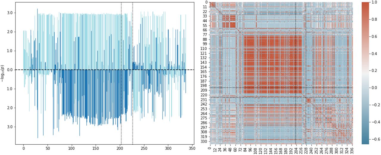
For illustration, we show the spectrum of SNPs considered in the CCR3 region and their SNP-SNP correlation in figure 8. The correlation between SNPs is clearly visible. Note that the SNPs are in high LD, as is evident from the heatmap shown on the right hand side of figure 8. Using the method described in section IV, we calculate a p-value of 1.50 × 10⁻⁸ for the significance of the coherence.

Left: SNP p-values after rank transform for the CCR3 gene. The x-axis is numbered according to the ith SNP in the gene window ordered by increasing position. The dotted black lines indicate the transcription start and end positions (first and last SNP). Up bars correspond to M05B and down bars to severe Covid-19. Light blue indicates positive and dark blue negative association. Right: SNP-SNP correlation matrix inferred from the 1KG reference panel.
Note that the chemokine receptor of type 1 is involved in regulation of bone mineralization and immune/inflammatory response. In particular, chemokines and their receptors are critical for recruitment of effector immune cells to the location of inflammation. Mouse studies suggest that this gene plays a role in protection from inflammatory response and host defence [26, 27].
The SNP spectrum in the LZTFL1 region is shown in figure 9. In contrast to the gene discussed above, LZTFL1 contains several independent LD blocks. The p-value for the significance of the covariance is calculated to be given by 1.19 × 10⁻⁷. Additional indications for the observed co-signficance of LZTFL1 for the two traits may be found in that it is known that the gene LZTFL1 modulates T-cell activation and enhances IL-5 production [28]. In particular, mouse models suggest that expression of IL-5 alters bone metabolism [29].

Left: SNP p-values after rank transform for the LZTFL1 gene. Annotation as in figure 8. Right: SNP-SNP correlation matrix inferred from the 1KG reference panel. Note that the gene contains independent LD blocks.
Direction of association and coherence suggests that genetic predispositions leading to M05B intake may carry a higher risk for severe Covid-19, with shared functional pathways related to the genes discussed above.
b. Anti-coherence
We perform a similar test between Covid-19 severity and drug classes as above for anti-coherence. The corresponding results for all medication classes are shown in figure 6. Despite the fact that no drug class possesses a Bonferroni significant hit, we note that the drug classes H03A (Thyroid preparations), C10AA (HMG CoA reductase inhibitors), L04 (Immunosuppressants) and M01A (Anti-inflammatory and anti-rheumatic products) have gene hits with a p-value < 1 × 10⁻⁵. All of these drugs find applications in auto-immune diseases and allergies. The genes with a p-value below 1 × 10⁻⁵ for H03A are HLA-DQB1, for C10AA SMARCA4 and BCAT2, for L04 LZTFL1, TRIM10, TRIM15 and TRIM26, and for M01A TRIM10 and TRIM31. Note that TRIM proteins are involved in pathogen-recognition and host defence [30]. For illustration of the anti-coherence case, we plot the SNP spectrum for TRIM10 under L04 in figure 10. We tested the above genes for direction of aggregated effect sizes under the Covid-19 GWAS via (16) and found that the detected genes for H03A, L04 and M01A tend to be localized in the left tail. Hence, a protective effect is suggested for these genes and therefore conditions leading to intake of these medications may imply a lower genetic risk for severe Covid-19.
Left: SNP p-values after rank transform for the TRIM10 gene under medication L04. Annotation as in figure 8, but up bars corresponding to L04. Right: SNP-SNP correlation matrix inferred from the 1KG reference panel.
c. M05B related traits
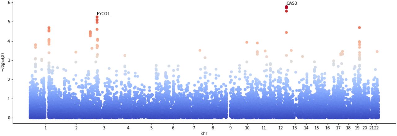
The main application of M05B medications is the treatment of Osteoporosis. In order to investigate this potential link further, we cross score the Covid-19 GWAS against a selection of GWAS with phenotypes related to Osteoporosis. Namely, bone mineral density (BMD) estimated from quantitative heel ultrasounds and fractures [31], Estrogene levels in men (Estradiol and Estrone) [32], Calcium concentration [33], Vitamin D (25OHD) concentration [34] and Rheumatoid Arthritis [35]. The inferred gene enrichment for coherence and anti-coherence with the Covid-19 GWAS is shown in figure 11. We find enrichment with gene p-values < 10−5 for Vitamin D and Calcium. In particular, in the anti-coherent case the most significant genes for Vitamin D are OAS3, OAS2, OAS1, FYCO1, CXCR6 and LZTFL1. We show the corresponding Manhattan plot in figure 12. The OAS family are essential proteins involved in the innate immune response to viral infection. They are involved in viral RNA degradation and the inhibition of viral replication [36]. The gene CXCR6 (p = 7.96 × 10⁻⁶) is expressed by subsets of TH1 cells, but not by TH2 cells. The D-test shows that all these genes are in the right tail and therefore suggest an increase in the risk for severe Covid-19 under variations in these genes. In particular, the anti-coherence of CXCR6 towards Vitamin D concentration hints at that predisposition for Vitamin D concentration is linked to differences in immune system reaction, i.e., between type 1 (inflammatory) or type 2 (anti-inflammatory). Indeed, possible links between severity of Covid-19 and Vitamin D are actively discussed in the current literature. See for instance [37–39] and references therein.

Resulting p-values for cross scoring several GWAS related to Osteoporosis against the severe Covid-19 GWAS. We observe enrichment in Vitamin D and Calcium with several p-values < 10−5. The leading genes are indicated.

Manhattan plot for cross scoring Vitamin D concentration against severe Covid-19 in the anti-coherent case.
For Calcium the top genes are HGFAC (p = 4.15 × 10⁻⁷) and DOK7 (p = 1.61 × 10⁻⁶). Note that HGFAC is Bonferroni significant under the seven traits tested. Both genes sit in the left tail under the D-test (16) applied to the Covid-19 GWAS. Therefore, for theses genes predisposition for high Calcium concentration suggest a reduced risk for severe Covid-19. Note that in general its is known that viruses appropriate or interrupt Ca2+ signaling pathways and dependent processes, cf., [40].
The gene HGFAC plays a role in converting hepatocyte growth factor (HGF) to its active form. In particular, binding of HGF causes the upregulation of CXCR3, which is primarily activated on T lymphocytes and NK cells. CXCR3 is preferentially expressed on TH1 cells, while CCR3 on TH2 cells [41]. In detail, CXCR3 binds the chemokine receptor CCR3 and prevents an activation of TH2-lymphocites. Thereby, a towards TH1 biased inflammation immune reaction is triggered [42]. Note that CXCR3 is able to increase intracellular Ca2+ levels [43].
The gene DOK7 is of importance for neuromuscular synaptogenesis. It activates MuSK, which is essential for maintenance of the neuromuscular junction as it is involved in concentrating AChR in the muscle membrane at the neuromuscular junction. The latter protein is critical for signaling between nerve and muscle cells, a necessity for movement. Hence, it may be possible that DOK7 could be involved in a genetic explanation of the muscle weakness impacting some of the severe Covid-19 patients [44].
Note that for the Vitamin D and Calcium GWAS, we observe cross enrichment in, both, the coherent and anti-coherent case with the severe Covid-19 GWAS, cf., figure 11. For example, for Vitamin D one implied coherent gene of potential interest is OS9 (p = 4.2 × 10⁻⁶). The corresponding protein binds to the hypoxia-inducible factor 1 (HIF-1). HIF-1 is a key regulator of the hypoxic response. In particular, regulation of HIF-1 interpolates between regeneration and scaring of injured tissue. It is known that severe Covid-19 may lead to lung tissue fibrosis. The D-test applied to the Covid-19 GWAS shows that OS9 is located in the left tail and therefore a protective property of variations in this gene are suggested.
2. Comparison to baseline
It is illuminative to compare to a more simple way to detect potential co-significance of a gene for two GWAS. Namely, we may simply compute gene trait significance values via the original Pascal methodology, i.e., making use of (14), and using gene-wise product-normal significance thresholds to detect genes of interest. Note that in doing so we ignore coherence of the SNPs inside the gene, and thereby compare only the total amount of variation. As before, we use jointly QQ-normalized GWAS p-values to suppress unintended uplift. Figure 13 (top plot) shows the scatter plot for gene-wise log-transformed p-values for the severe Covid-19 GWAS against the medication class M05B GWAS, and significance thresholds for the product-normal. We observe that in this example the simple approach is consistent with the results of the more elaborate cross-scoring of the previous section. In particular, the genes CCR1 and CCR3 are confirmed to be of interest for both traits. Similar observations can be made for plotting the gene scores of severe Covid-19 against Vitamin D concentration, see figure 13 (middle plot).
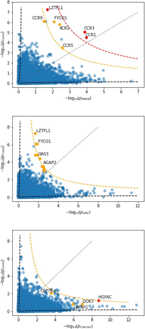
GWAS gene scores, obtained separately for two GWAS using joint QQ-normalization and (14), plotted against each other. Each point corresponds to a gene. Top: Covid-19 vs. M05B. Middle: Covid-19 vs. Vitamin D. Bottom: Covid-19 vs. Calcium. The gray dotted line marks the diagonal. The orange and red dashed curves mark the gene-wise product-normal threshold curves for significance of 10−5, respectively, 10−7. The color of a gene (red and orange) indicate the SNP-wise cross scored p-value (< 10−6, respectively, < 10−5). The black dashed curves indicate significance threshold curves of 10−2 for the ratio test.
In general, we would expect that the simple approach described in this section would lead to more false positives, but would also lead to false negatives. The danger for false positives is clear, as the simple approach is blind to incoherent directions of association between the SNPs of the two GWAS in the gene window under consideration. However, also false negatives may occur: In the proposed novel approach using (15), several independent weak signals may combine to a stronger signal, if the directions of association are consistent over the gene window. Such signals are invisible in the simple approach of comparing aggregated gene p-values. That this is not only hypothetical may be seen at hand of figure 13 (bottom plot), there a gene p-value scatter plot is shown for severe Covid-19 against Calcium concentration. Remarkably, the detailed approach using individual SNP information marks genes to be of interest which are away from the gene-wise significant curve, and ignores other genes which are closer.
3. Ratio test
Let us also briefly discuss an application of the ratio based causality test introduced in sections V and VII Ae. For illustration, ratio test significance threshold curves for p = 10−2 are indicated in figure 13. Note that the genes of non-interest are generally located between the two types of significance curves (in the figure between the black and orange dashed curves). Genes of relevance for the ratio test are instead engulfed by the coordinate axis and the ratio significance threshold curve (black dashed curves).
We ratio tested the Covid-19 GWAS against the Vitamin D and Calcium concentration GWAS in the coherent case and found that Vitamin D carries an interesting hit which suggests a causal pathway from genetic predisposition for Vitamin D concentration to severity of Covid-19. The ratio test Manhattan plot is shown in figure 14. In particular, besides the genes KLC1 and AL139300.1, the gene ZFYVE21 (pR = 3.9 × 10⁻⁶) stands out. Under the Covid-19 GWAS (outcome) the gene carries a p-value of pV = 0.99 while under the Vitamin D GWAS (exposure) a p-value of pV = 6.5 × 10⁻⁴. This implies a causal flow from genetic predisposition for Vitamin D concentration to severity of Covid-19. We confirmed that Calcium concentration is not a potential confounder for ZFYVE21 (pV = 0.26). The D-test shows that the gene is in the right tail and hence is associated with high Vitamin D concentration. A possible explanation of the hit may go as follows. ZFYVE21 regulates microtubule-induced PTK2/FAK1 dephosphorylation, which is important for integrin beta-1/ITGB1 cell surface expression. It has been discussed before in the literature that integrins in host cells may play the role of alternative receptors to ACE2 for SARS-CoV-2 [45, 46]. Hence, it is tempting to speculate that genetic predisposition for Vitamin D concentration may also influence expression of the integrin receptors, and thereby the outcome of Covid-19 via an increased risk of cellular infection.

Manhattan plot for ratio scoring Vitamin D concentration against severe Covid-19 in the coherent case, with ratio denominator given by Covid-19.
Another gene we observe to be of relevance in the coherent case is the Ring Finger Protein 217 (RNF217) with pR = 1.83 × 10⁻⁶ and Calcium as exposure. We have pV = 2.15 × 10⁻⁵ under Calcium and pV = 0.82 under Covid-19. The gene is associated with low Calcium concentration, as the D-test implies (left tail). The potential role played by this gene in the Covid-19 context is however unknown. As the gene shows an illustrative coherence pattern (multiple LD blocks), we show the corresponding SNP correlation plot in figure 15.

Left: SNP p-values after rank transform for the RNF217 gene under Calcium concentration and severe Covid-19. Annotation as in figure 8, but up bars corresponding to Calcium. Right: SNP-SNP correlation matrix inferred from the 1KG reference panel.
We also tested the anti-coherent case. The gene HOXC4 with pR = 4.5 × 10⁻⁶ is detected for M05B. Individual scored p-values for the gene read pV = 2.04 × 10⁻⁵ under M05B and pV = 0.75 under Covid-19. The D-test under M05B shows that the gene signal is located in the left tail. Hence, modulo potential confounders, a causal relation from predisposition to take M05B to a protective property towards severity of Covid-19 via HOXC4 is suggested. We note that HOXC4 has been discussed before in the Covid-19 context [47]. The gene is related to an enhanced antibody response under the regulation of estrogens. This matches the observation of anti-coherence with severity of Covid-19.
Interestingly, also for the inverse causal relation, i.e., a predisposition for severe Covid-19 implying a predisposition for the need to take M05B medication, a relevant gene is singled out. Namely, the gene DDP9 with pR = 3.88 × 10⁻⁵, and pV = 0.74 under M05B, respectively, pV = 2.57 × 10⁻⁵ under Covid-19. This gene has been implicated before to be involved in the genetic mechanisms for critical illness due to Covid-19 [48]. Note that we also observe DPP9 (pR = 5.82 × 10⁻⁷) as top hit for Calcium concentration as exposure, cf., the corresponding Manhattan plot shown in figure 16. Under both exposures the gene signal tends to be more in the right tail of the D-test. Another gene we detect in this ratio test is IFNAR2 (pR = 9.70 × 10⁻⁶), a known possible drug target against Covid-19 [48]. Note that this gene appears to be in the left tail of the D-test under Calcium as exposure.

Manhattan plot for ratio scoring Calcium concentration against severe Covid-19 in the anti-coherent case, with ratio denominator (outcome) given by Calcium concentration.
For Vitamin D as exposure, we find in the anti-coherent case that the genes MED23 (pR = 5.22 × 10⁻⁵ and GATA4 (pR = 7.88 × 10⁻⁵) are the leading hits with a p-value < 10−4. The D-test shows that MED23 is in the right tail under the exposure, whereas the test is in-conclusive for GATA4. The Mediator subunit MED23 occurred before in SARS-CoV-2 screens, with a critical role of this complex during infection and death suggested [49]. GATA4 has been observed previously in the context of the top significant biological processes likely associated with respiratory failure in Covid-19 patients [50].
Finally, note that we pick up the genes HGFAC (pR = 4.2 × 10⁻⁵ and DOK7 (pR = 1.27 × 10⁻⁵), already detected before via the coherence test, as well via the anti-coherent ratio test with Calcium as exposure, suggesting a causal pathway. In addition, we observe for Calcium as exposure the leading gene PPP2R3A (pR = 1.0 × 10⁻⁵), with unknown relation to Covid-19.
VIII. SUMMARY AND CONCLUSION
The core technical observation of this paper can be found in equations (5) and (B4), expressing the product-normal and variance-gamma distribution in terms of a χ2 difference distribution. This allows for efficient calculation of the corresponding cdf and tail probabilities with Davies algorithm. This also allows one to perform a significance test of covariance for dependent samples, as long as the inter-sample correlation structure is known, see equation (8). Davies algorithm as well allows the calculation of the cdf of the ratio distribution (9), which finds application in testing for a causal relation.
We discussed a potential application for GWAS. Namely, to find coherent genes between different traits, cf., section VII. We applied this method to uncover a potential link between severe Covid-19 and underlying conditions leading to usage of medications of class M05B. We found that chemokine receptors play a major role. Further investigations at hand of related GWAS phenotypes revealed genetic links to Vitamin D and Calcium concentrations, with Covid-19 cross implicated genes related to differentation between type 1 and type 2 immune response. A possible explanation of this emerging link being that patients taking class M05B medication usually suffer under Osteoporosis. Vitamin D stimulates the absorption of Calcium and therefore is related to bone mineral density [51]. However, it is also well known that Vitamin D contributes to reducing the risk of infection and death, mainly due to factors involving physical barriers, cellular natural immunity and adaptive immunity [52]. In this work we found hints that also the severity of Covid-19 may be impacted by Vitamin D concentration via influencing the immune response by pathways including chemokine receptors. In addition, we detected a potential causal link from genetic predisposition for Vitamin D concentration to severity of Covid-19, mediated by the ZFYVE21 gene, which is related to integrin beta-1/ITGB1 cell surface expression and thereby potentially impacting disease outcome by influencing alternative receptors to ACE2 for host cell entry.
The previously in the severe Covid-19 context observed genes HOXC4 and DPP9 are also detected by our method, with a potential causal link to conditions leading to M05B medication intake. Similarly for MED23 and GATA4 with a potential causal link from Vitamin D concentration predisposition. Note that we can not exclude potential confounders.
We also found that genetic variants in genes related to both the adaptive (HLA) and innate immune system (TRIM genes) that have a higher frequency in subjects taking medications indicated for specific auto-immune disorders tend to reduce the risk of severe Covid-19. Indeed, it is well known that auto-immune disorders are more common in females, who also have a smaller risk of severe Covid-19 in comparison to men. While it is of course reasonable to expect that subjects with an increased risk for auto-immune disorders will tend to fight off infections more efficiently, the added value of our analysis is to pinpoint specific genes that are potentially involved in mediating this effect, and which may hint towards a protective and/or therapeutic pathway against severe Covid-19.
In general, we find it astonishing that the relatively simple methods presented in this work produce leading gene hits of apparently very high plausibility, and also re-discovers genes previously indicated in the literature. We therefore believe that the methods presented in this work may find wider utility.
Note that it is not a contradiction that we find the possibility for in effect diverging pathways between different genes for a pair of traits. It rather illustrates that in general the influence of one trait onto the other is a complicated interplay between in direction competing effects. More naive, full genome based, methods like genetic correlation or usual applications of Mendelian randomization can not resolve this fine structure, but rather yield only an aggregated trend for the traits. We therefore like to stress that statements made in this work regarding trait risk implications are not made for the traits in general, but rather for the respective gene under discussion. For a given pair of traits, the implication may differ between different genes.
In this work we assumed that there is no sample overlap between the GWAS under consideration and that the GWAS under consideration either have similar sample sizes, or that effects of sample sizes differences can be compensated by QQ-normalization. It would be interesting to study the potential impact of sample overlap in more detail and explicitly include the possibility for different sample sizes in the discussion of section VII. Artifacts of sample overlap could perhaps be corrected along the lines of [53, 54].
We can envisage other, more general, applications of the methods discussed in this paper. For instance, the methods might be of use to correct for the auto-correlation structures in estimating the significance of correlation between time-series. Hence, the technical results of this paper may be as well of interest for other domains.
Data Availability
All data is publicly available from third-parties in terms of summary statistics and references given.
Acknowledgments
We like to thank A. L. Button, A. Brümmer, Z. Kutalik and S. O. Vela for valuable comments on an earlier draft of the manuscript.
appendix A General product-normal
Let us briefly consider as well the distribution for xy with  and
and  , i.e., the product-normal for non-standardized Gaussian random variables. The moment generating function reads [19]
 Note that for, either, µx = 0 or µy = 0, the factorization of the main text still holds. Defining
  and
and  , the exponent of the exponential in
  can be split for the general non-correlated case (ϱ = 0) into
 We deduce that we can still factorize the moment generating function, such that
 with
with  the non-central χ2 distribution with one degree of freedom. Hence, the general product-normal can be expressed as a linear combination of non-central
  distributions, for ϱ = 0.
Appendix B Probability density functions
a. Product-Normal
Making use of the relation (4), the pdf, denoted as f, of the product-normal distribution can be calculated analytically via convolution (cf., [55])
 Completing the square and invoking hyperbolic substitution, we arrive at
 with K0 the modified Bessel function of second kind at zero order. The result above for f is in agreement with the previous derivations of [56, 57]. Note that the analytic calculation of the corresponding cdf requires the solution of an integral of the type
  . We are not aware of a known closed form solution.
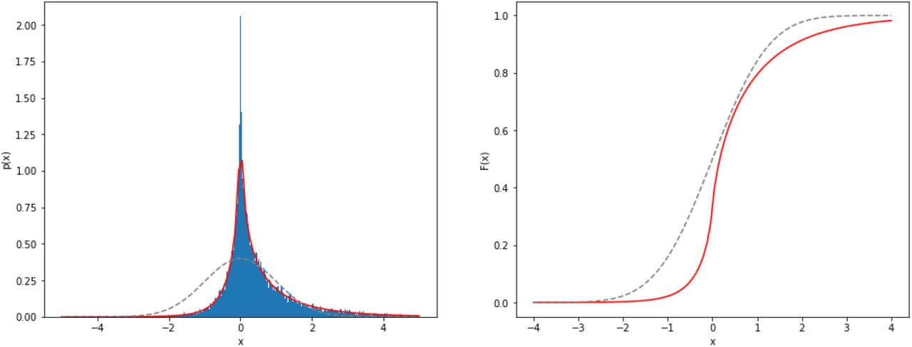
For illustration, we plot the pdf for ϱ = 1/2 together with the corresponding histogram sampled from (4) in figure 17. We also show the cdf obtained via numerical integration of (B1). We verified that the numerical integration matches the results obtained via Davies algorithm for the cdf calculation for various ϱ, cf., table I.
Mean squared error (MSE) between numerical integration of (B1) and Davies algorithm for various ϱ and 1000 arguments evenly spaced in the range [−4, 4].

Left: Histogram of the dependent product normal distribution with ρ = 0.5 obtained via subtracting 50.000 pairs of random samples of Gamma distributions following (4). The red line marks the pdf given in (B1). Right: The corresponding cdf obtained via Davies algorithm. For comparision, the dashed gray lines show the corresponding normal quantities.
Note that since the pdf of the non-central χ2 distribution includes a Bessel function, analytic calculation of the pdf of xy in the more general case of section A is more complicated than in (B1), and will not be discussed here.
b. Variance-Gamma
Consider a random variable X distributed according to
 The corresponding pdf can be calculated similar as above via convolution. We infer
 Completing the square and using as before hyperbolic substitution, we arrive at
 with Kn a modified Bessel function of second kind at order n. Using the integral
  , we easily verify that
  Hence, due to symmetry the pdf is well normalized. However, we are not aware of closed form solutions for Bessel function integrals of the type
  , which are needed to provide a closed form expression for the cdf.
The distribution given by (B3) occurred before in the finance domain as a special case of the Variance-Gamma distribution [58]. It can be traced back further to the distribution of the bivariate correlation. In detail, the gamma-variance corresponds to the off-diagonal marginal of a two-dimensional Wishart distribution, which models the covariance matrix [59]. However, what is new, to the best of our knowledge, is the expression in terms of the difference distribution in equation (B2).
For h = n and g = 1, we have
 Hence, for n = 1 we obtain the product-normal distribution with ϱ = 0 as discussed in the previous section. For general n we can view X(n, 1) as the distribution of a sum of n independently distributed product-normal random variables. In particular, we can make use of Davies algorithm to calculate the cdf for X(n, 1) exactly at a desired precision.
References
- [1].↵
- [2].↵
- [3].↵
- [4].↵
- [5].↵
- [6].↵
- [7].↵
- [8].↵
- [9].↵
- [10].↵
- [11].↵
- [12].
- [13].↵
- [14].↵
- [15].↵
- [16].↵
- [17].↵
- [18].↵
- [19].↵
- [20].↵
- [21].↵
- [22].↵
- [23].↵
- [24].↵
- [25].↵
- [26].↵
- [27].↵
- [28].↵
- [29].↵
- [30].↵
- [31].↵
- [32].↵
- [33].↵
- [34].↵
- [35].↵
- [36].↵
- [37].↵
- [38].
- [39].↵
- [40].↵
- [41].↵
- [42].↵
- [43].↵
- [44].↵
- [45].↵
- [46].↵
- [47].↵
- [48].↵
- [49].↵
- [50].↵
- [51].↵
- [52].↵
- [53].↵
- [54].↵
- [55].↵
- [56].↵
- [57].↵
- [58].↵
- [59].↵


