
Abstract
The concentration of SARS-CoV-2 RNA in faeces is not well established, posing challenges for wastewater-based surveillance of COVID-19 and risk assessments of environmental transmission. We develop versatile hierarchical models for faecal RNA shedding and apply them to data collected in six studies. We find that the mean number of gene copies per mL of faeces is 1.9×10⁶ (2.3×10⁵—2.0×10⁸ 95% credible interval) amongst hospitalised patients. We find no evidence for a subpopulation of patients who do not shed RNA: limits of quantification can account for negative stool samples. Our models indicate that hospitalised patients represent the tail of the shedding profile with a half-life of 34 hours (28—43 95% credible interval), suggesting that wastewater-based surveillance signals are more indicative of incidence than prevalence and can be a leading indicator of clinical presentation. Shedding amongst inpatients cannot explain high RNA concentrations observed in wastewater, consistent with more abundant shedding during the early infection course.
1. Introduction
The novel virus SARS-CoV-2 (severe acute respiratory syndrome coronavirus 2) infected over 80 million people in 2020, and more than 2.6 million people have succumbed to the resultant disease, COVID-19 (coronavirus disease 2019) [1]. Individuals infected by the virus primarily suffer from respiratory symptoms [2], but gastrointestinal manifestations of the disease have also been observed [3]. The presence of viral RNA in faeces allows for the surveillance of COVID-19 by quantifying gene copies in sewage [4]. So-called wastewater-based epidemiology (WBE) provides data that can complement traditional testing schemes and can be used to monitor the disease relatively cheaply by pooling wastewater from thousands of people [5]. Correlations between case numbers from individual testing schemes and RNA concentrations in wastewater have been observed [4, 6, 7]. However, associative studies cannot easily be used to calibrate WBE approaches: each sewerage system is different [8], and case numbers may not be a good indicator of prevalence [9]—especially when testing capacity is limited. The World Health Organisation considers “quantitative information on viral shedding” an imminent need to reap the potential benefits of WBE [10].
Faecal shedding of RNA suggests that the virus could be transmissible via the faecaloral route [11]. While presence of RNA does not imply presence of infective virus, the likelihood increases with higher RNA loads [12]. Sewer overflows could cause spillover events, leading to new viral reservoirs [13]. For example, mink are susceptible to SARS-CoV-2 [14] and can be exposed to untreated sewage [13]. Furthermore, wastewater workers are at risk of contracting sewage-borne pathogens [15], and wastewater is a possible infection mode in densely populated communities [16, 17]. Quantifying these risks is essential for making informed policy decisions.
We developed a family of random-effect models [18, ch. 5] for SARS-CoV-2 RNA concentrations in faecal samples and applied them to data from six clinical studies to study three aspects of faecal RNA shedding. First, we studied the shedding profile, i.e. the temporal variability of shedding over the infection course, which affects the interpretation of WBE results [6]. We find that the profile decays quickly with a half-life of 34 hours. Second, the proportion of patients with one or more positive faecal samples has been extensively studied [3, 19, 20]. We determined that the limit of quantification of assays can account for patients without positive samples. Bayesian model comparison revealed no evidence for a subpopulation of patients who do not shed RNA faecally. Third, we obtained estimates of the mean faecal RNA concentration: a quantity important for inferring disease prevalence or incidence from wastewater data [21]. We show that the models are able to predict summary statistics of held-out studies accurately and consider the implications of our results for wastewater-based epidemiology.
2. Results
To study faecal RNA shedding quantitatively, we developed a suite of hierarchical models for RNA concentrations in faecal samples, as described in section 4.1. In contrast to existing quantitative approaches [22, 23], our models can account for a variable number of samples per patient, incorporate data from studies with different levels of quantification, and capture variability between patients as well as variability between samples from the same patient. The baseline model assumes that all infected patients shed viral RNA faecally and that typical RNA concentrations in samples vary over the course of the infection. We considered three different shedding profiles: an exponential decay profile, a gamma profile, and the exponential rise-and-decay profile proposed by Teunis et al. [24] for norovirus RNA shedding (see section 4.1.1 for details). We call this the temporal standard model, and it is illustrated in fig. 1.

The population-level distribution (shown in blue) captures variation in shedding behaviour between patients, giving rise to location parameters µi for each patient i (see section 4.1 for details). The location parameters (blue squares) describe the amplitude of individual shedding profiles as illustrated for three patients. The patient-level distribution (shown in orange for one patient) describes the variation between samples from the same patient, and the shedding profile (solid black line) modulates typical RNA concentrations in faecal samples over time. All samples are analysed using an RT-qPCR assay with a given limit of quantification (LOQ) θ (dashed black line), and concentrations above the LOQ (orange circles) can be quantified. Concentrations below the LOQ (orange cross) cannot be quantified. Currently available data do not allow us to constrain the early shedding profile, and late-stage shedding is consistent with an exponential decay profile.
We considered two modifications to the baseline model. First, we considered a constant model, where the time-variability of shedding was removed. Second, to assess whether there exists a subpopulation of patients who never shed viral RNA faecally, we introduced a shedding prevalence parameter ρ such that all samples of an infected patient are negative with probability 1 − ρ. We call this the subpopulation model (as opposed to the standard model in which all patients shed RNA faecally). Combining the two modifications (with and without a subpopulation of non-shedders, and with and without time-variability) gives rise to four models in total.
We fitted each model to longitudinal data extracted from three studies [26, 25, 12] listed in table 1. All studies used RT-qPCR assays to quantify SARS-CoV-2 RNA copies in faecal samples collected from hospitalised patients. The two constant models were also fitted to an additional dataset collected by Wang et al. [11] that does not provide temporal information. As shown in table 2, we compared the models using the Bayesian model evidence [29] (i.e. the marginal likelihood of the data under each model), allowing us to draw two conclusions.
Microdata, i.e. sample-level RNA concentrations, provided by the first four studies were used to fit random effects models. The next two studies did not provide microdata, and we validated our models by comparing reported summary statistics with model-based predictions, as discussed in section 4.4. Samples with viral loads below the limit of quantification (LOQ) are considered negative for SARS-CoV-2. The table also reports the total number of patients n and number of samples m, including a breakdown by positivity.
Model evidences evaluated on three common datasets prefer temporal models (evidence shown for an exponential decay profile) over constant ones, and standard models are preferred over models with a subpopulation of patients who do not shed SARS-CoV-2 RNA faecally. Parameter estimates are consistent with conclusions based on model evidences. They are reported as the posterior mode together with the 95% credible interval in brackets. All reported credible intervals are highest posterior density intervals. Estimates for constant models include a fourth dataset without temporal information.
First, accounting for the time dependence of the shedding profile is essential. The three shedding profiles we considered are indistinguishable where data are available to constrain them (see section 4.1.1 for details). However, there are only few samples obtained prior to day six past symptom onset, as shown in fig. 2 (a), and shedding behaviour during the early infection course cannot be constrained given the available data. For simplicity, we use the exponential decay profile unless otherwise specified. Typical faecal RNA concentrations decay with a maximum a posteriori half-life of 34 hours (28—43 hours 95% credible interval) amongst hospitalised patients, as shown in fig. 2 (b) and (c).

Panel (a) shows a histogram of the number of samples collected on each day post symp-tom onset. The small number of samples collected within the first six days after symptom onset and the absence of samples collected prior to symptom onset make it difficult to constrain shedding during the early infection course. Panel (b) shows longitudinal faecal RNA concentration data from three studies together with the level of quantification for each study as dashed lines. The time-dependent exponential shedding profile of the temporal standard model is shown in black, and the shaded region represents the 95% credible interval of the profile (see section 4.1 for details). Panel (c) shows the posterior distribution for the half-life τ1/2 of the shedding profile.
Patients may not recall the number of days since symptom onset accurately, or they may present with atypical symptoms that are not easily identified as the onset of COVID-19 [30]. To assess the sensitivity of the inferred half-life to inaccurate reports, we repeated the inference after adding up to three days of reporting noise to the number of days since symptom onset. No sensitivity of the half-life inference to inaccurate reports was observed.
The second result is that there is no evidence for a subpopulation of patients who do not shed viral RNA faecally; standard models (without a non-shedding subpopulation) are preferred for both the constant (log odds of 3.1 ± 0.3) and temporal models (log odds of 1.8 ± 0.3). Consistent with the model comparison results, the inferred shedding prevalence is large and the 95% credible interval includes ρ = 1 for both subpopulation models. Consequently, as discussed in more depth in section 4.4, the level of quantification of the assays used in the three studies can explain the number of negative patients and samples because “the level of viral RNA present in stool can fluctuate around the margin of laboratory detection” [28].
To assess the out-of-sample predictive utility of the models, we considered predictions for two held-out datasets that do not provide microdata, as listed in table 1. The studies conducted by Kim et al. [27] and Ng et al. [28] provided sufficiently detailed descriptions of their protocols to simulate the studies and make predictions by sampling from the posterior predictive distribution (see section 4.4 for details). Since our models have not been fit to these data, their ability to predict summary statistics of those data is an indication of how well the models generalise. Temporal models are preferred by the data, but we do not have any temporal information about the studies conducted by Kim et al. [27] and Ng et al. [28]. Nonetheless, the constant models can make accurate out-of-sample predictions because all studies consider the same population: hospitalized patients.
Kim et al. [27] collected 129 samples from 38 hospitalised patients, and they reported the largest observed concentration max x = 2.7 × 10⁷ gene copies per mL of faeces. Ng et al. [28] collected 81 samples from 21 patients, and the largest observed RNA concentration was max x = 1.3 × 10⁷ copies per mL. As shown in fig. 3 (a) and (b), predictions from our models are consistent with the reported values. Predictions of the maximum are smaller for the study by Ng et al. [28] than Kim et al. [27], which is expected owing to a smaller number of samples (so the tails of the distribution are less well sampled). Ng et al. [28] also reported the median number of positive samples per patient median m•(+). Because they report the limit of detection of their assay, we can make predictions about the median number of positive samples per patient which agree with the reported value, as shown in panel (c) of fig. 3.

Predictions of the maximum concentration observed by Kim et al. [27] and Ng et al. [28] are shown in panels (a) and (b) as violin plots, respectively. The value reported in the studies is shown as black dashed lines. Panel (c) shows predictions of the median number of positive samples per patient reported by Ng et al. [28]. Only results for the constant models are shown because the two studies did not provide temporal information.
3. Discussion
We have inferred properties of the faecal SARS-CoV-2 RNA shedding distribution by fitting a suite of Bayesian hierarchical models to clinical data from four studies. The models account for the limits of quantification of RT-qPCR assays and a variable number of samples per patient. They are able to capture salient properties of the data and generalise well to two held-out datasets. There is no evidence of patients who do not shed viral RNA faecally.
The inferred temporal shedding profile is robust to inaccurate reports of the number of days since symptom onset, and it suggests that hospitalised patients are in the tail of the shedding profile because faecal RNA concentrations decay by an order of magnitude over the course of four to five days. While extrapolation should be treated with caution, wastewater-based surveillance of COVID-19 lends additional credibility to the hypothesis that SARS-CoV-2 RNA concentrations in wastewater are higher than expected based on faecal shedding inferred from hospitalised patients [31]. Assuming mean faecal RNA concentrations Λ are not larger in mild cases in the community than amongst hospitalised patients, a daily per capita wastewater volume of V = 300 L [32], and faecal mass of m = 128 g per person per day [33], we would expect wastewater RNA concentrations on the order of mΛ/V ~ 103 mL−1 if every person was infected. In practice, concentrations in excess of 103 mL−1 have been observed [4] at times when seroprevalence of SARS-CoV-2 antibodies was less than ten percent [9]. Substantial shedding during the early stages of the infection likely explains these observations. The rapid decay of the shedding profile also implies that signals from wastewater-based surveillance of SARS-CoV-2 are likely more indicative of incidence, rather than prevalence. Wastewater-based surveillance is thus a promising approach for early detection of cases in the community. A better understanding of the shape of the shedding profile, including prior to symptom onset, is essential for interpreting signals from WBE correctly during critical phases of rapid changes in levels of infection.
While one of the largest quantitative studies revealed no association between disease severity and faecal RNA concentration [34], results obtained from hospitalised patients are unlikely to apply to the general population, e.g. the former tend to be older and have more comorbidities. Faecal samples should be collected from a representative sample of patients over the entire infection course to refine quantitative estimates of faecal shedding of SARS-CoV-2 RNA. These data should include faecal volumes to estimate the total RNA load in faeces in addition to concentrations. The effect of vaccinations and emerging variants on faecal RNA shedding should also be investigated to make wastewater-based surveillance an effective quantitative monitoring tool.
4. Methods
4.1. Models
We developed a suite of hierarchical models to characterise faecal shedding of SARS-CoV-2 RNA quantitatively. Starting with the standard constant model described in section 2, we discuss the generative model in three steps.
First, the mean faecal RNA concentration λi for each patient i ∈ {1, …, n} follows a distribution with probability density function f, where n is the number of patients. Log-normal, Weibull, and gamma distributions are common choices for distributions that model positive, continuous data [35]. However, conclusions based on these distributions can differ substantially due to their tail behaviour [36]. We thus employed a generalised gamma distribution (GGD) with shape Q, location M, and scale S. The GGD is a flexible distribution which encompasses the log-normal distribution (Q = 0), Weibull distribution (Q = 1), and gamma distribution (Q = S) as special cases [37]. This choice comes at the cost of wider credible intervals, commensurate with our lack of prior knowledge about the shape of the shedding distribution.
Second, mi samples are collected from each patient i. The RNA concentration yij in sample j from patient i follows a GGD with shape q, location µi, and scale σ. For the constant model (without time-varying shedding), the location parameter µ for the patient-level distribution is chosen such that ⟨yij⟩= λi for each patient. Because of the properties of the generalised gamma distribution, we can express the location parameter in terms of the mean as
 where Γ denotes the gamma function (see appendix A for details).
Third, the RNA concentration yij is quantified using an assay with level of quantification (LOQ) θij (see Kitajima et al. [38] for an overview of different assays). If the concentration is below the LOQ, the sample is considered negative for the purpose of this study, and we denote the output of the assay as xij = ∘. Otherwise, the result of the assay faithfully captures the RNA concentration in the sample, i.e. xij = yij. We do not explicitly model measurement error or variability between technical replicates in this study because the relevant data are not available and assays tend to yield reproducible results. For example, the CDC N1 assay [39] has a coefficient of variation < 3.7%—much smaller than typical variability between samples from the same patient. The RNA quantification is censored by the LOQ, and the likelihood of observing a particular assay result xij is thus
 where f denotes the probability density function of the generalised gamma distribution and F denotes the corresponding cumulative distribution function [37].
4.1.1. Time-variation
RNA shedding varies over the course of the infection [40], and the constant model cannot capture these changes. We incorporate temporal variability by introducing a shedding profile such that the expected RNA concentration λi for each patient i varies over time. In particular, we let λi(t) = λi(t = 0)g(t), where t is the number of days since symptom onset, g(t) is the shedding profile that modulates the expected RNA concentration, and λi(t = 0) is sampled from the population-level distribution. The shape and scale parameters q and σ of the patient-level distribution are kept constant.
Because all available data were collected from hospitalised patients several days after the initial onset of symptoms, we can only constrain the later part of the shedding profile. We used an exponential profile gexp(t) = exp (−αt), where α is the decay rate of the profile, because it provides an adequate fit for late-stage faecal shedding of other viruses [24]. Substituting into eq. (1), the exponential shedding profile gives rise to a location parameter that varies linearly with the number of days after symptom onset for each patient i such that µi(t) = µi(t = 0) − αt.
Any reporting error associated with the number of days since symptom onset t can be compensated for by a corresponding change in µi(t = 0). This explains why the inferred shedding profile is robust to reporting inaccuracies, as discussed in section 2. The profile shown in fig. 2 (b) is exp (M − αt), and it captures the decay of the effective population-level location parameter M over time. The profile half life is  .
.
We also considered two further shedding profiles to assess the sensitivity of our infer-ences to the choice of g(t). First, we used a gamma shedding profile
 where α > 0 and β > 0 control the shape of the profile and t0 is the time at which shedding can first occur, i.e. g(t < t0) = 0. Second, we considered the exponential rise-and-decay profile proposed by Teunis et al. [24] for norovirus shedding
 where α and β control the rise and decay of the profile, respectively.
4.1.2. Non-shedding subpopulation
To investigate whether there is a subpopulation of patients who do not shed SARS-CoV-2 RNA faecally, we extended the model by introducing a binary indicator zi ∈ {0, 1} for each patient i. If zi = 1, the shedding behaviour of the patient is unchanged. If zi = 0, patient i does not shed RNA, and xij = ∘ for all samples j. The indicator variables follow a Bernoulli distribution with probability ρ, i.e. the prevalence of shedding amongst the population of patients. This extension gives rise to what we refer to as the subpopulation models.
We know that zi = 1 for any patient with one or more positive samples, and the likeli-hood follows eq. (2). However, for any patient i whose mi samples  are all below the LOQ, the likelihood is
 where the first term accounts for a patient who cannot shed RNA (zi = 0) and the second accounts for a patient whose samples are all below the LOQ (zi = 1).
4.2. Data acquisition
We searched the literature for primary research that reported quantitative information on SARS-CoV-2 RNA loads in faeces, and we identified eleven studies of interest [3, 11, 12, 26, 27, 28, 34, 41, 42, 43]. Semi-quantitative studies reporting only cycle-threshold values were excluded.
Data from four studies were used to fit the hierarchical models described in section 4.1. First, Wölfel et al. [12] reported longitudinal faecal RNA concentrations for nine patients in Munich who had been in close contact with a common index case. Second, Lui et al. [25] followed the first eleven patients hospitalised due to COVID-19 in Hong Kong. Third, Han et al. [26] studied the viral dynamics of a neonate and her mother in Seoul. Fourth, Wang et al. [11] reported cycle threshold (Ct) values of RT-qPCR assays for faecal samples from a subset of patients admitted to three hospitals in China, and we transformed Ct values to RNA concentrations using conversion constants provided in the publication. Longitudinal information was not available. Table 1 lists information on the number of patients and samples for each study.
Two studies provided summary statistics of viral RNA concentrations in faecal samples, such as the highest concentration observed, together with sufficiently detailed descriptions of the study design to replicate the studies in silico, as described in section 4.4. In particular, Kim et al. [27] quantified RNA concentrations in faecal samples collected from hospitalised patients, and Ng et al. [28] studied RNA concentrations in faecal samples to assess transmission risks associated with faecal microbiota transplants. These data are not used to fit the hierarchical models but instead to assess the out-of-sample predictive utility of our fitted models.
Five studies were excluded from the analysis despite providing quantitative information. First, using an assay originally developed for samples from ferrets [44], Jeong et al. [41] reported RNA concentrations of various specimen types, including faecal samples. However, the reported concentrations are orders of magnitude lower than reported in any of the other quantitative studies for any specimen type. Indeed, most measurements are below the limit of quantification of other studies. Second, Zhang et al. [42] reported detailed data in a figure, but it is not possible to extract the relevant information because of the low resolution of the figure, and the data could not be obtained by other means. Third, Zheng et al. [34] conducted a large study, comprising 85 patients and 842 faecal samples. Unfortunately, viral loads are only reported as the median for each patient (private communication). Finally, Pan et al. [43] and Cheung et al. [3] collected faecal RNA concentration data from 17 and 59 confirmed cases, respectively, but neither study provides information on the number of samples collected.
4.3. Parameter inference and model comparison
We used the nested sampler polychord [45] which draws samples from the posterior distribution and evaluates the model evidence, i.e. the marginal likelihood of the data under the model, as listed in table 2. The study by Wang et al. [11] was not used to estimate parameters for temporal models because longitudinal data were not available. Similarly, to facilitate a direct comparison between models, that study was also omitted from the evaluation of evidences. We used unit-scale half-Cauchy distributions for the shape parameters Q and q as well as the scale parameters S and σ. A flat prior on the interval 6—23 was used for the population location M which is sufficiently wide to avoid boundary effects. A flat prior on the unit interval was used for the shedding prevalence ρ. For models with temporal variability, a unit-scale Cauchy prior was used for the profile parameters α and β. We used uniform prior on the interval −14—7 for t0 such that the onset of shedding can differ from the onset of symptoms. All inferences were run in triplicate, and no sensitivity to different pseudo-random number generator seeds was observed (Gelman-Rubin diagnostic  1.05 for all models [46]).
In addition to the results discussed in section 2, we consider four technical implications of the inference here.
First, the gamma and Teunis shedding profiles are both consistent with the exponential shedding profile for late-stage shedding where data are available to constrain them. However, the available data cannot constrain early shedding behaviour, as illustrated by the wide range of shedding profiles consistent with the data shown in fig. 4. Miura et al. [22] reported tight posteriors for early shedding behaviour using the shedding profile proposed by Teunis et al. [24], but their inferences rely on the assumption that the time of symptom onset and shedding onset coincide (i.e. t0 = 0), an assumption that is not yet supported by evidence.

Panels (a) and (b) show the the posterior distributions for the time tpeak at which the inferred gamma and Teunis shedding profiles peak, respectively. Because the data cannot constrain early shedding, the posterior for tpeak has broad support. Panels (c) and (d) show posterior samples of the gamma and Teunis profiles, respectively, in blue. The exponential profile discussed in section 2 is shown as an orange line, and the shaded region corresponds to the 95% credible interval.
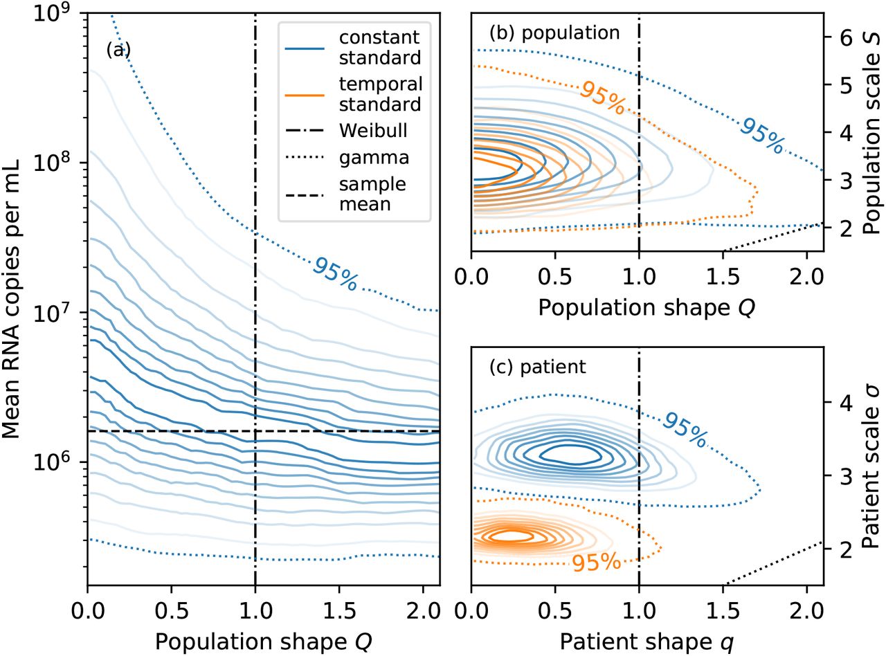
Second, the shape Q controls the tails of the population-level distribution: the larger Q, the lighter the tails (see Prentice [37] for details). The population-level mean RNA concentration, i.e. the expected RNA concentration in a random faecal sample from a previously unobserved patient, depends on the tail behaviour because the mean is sensitive to outliers [36]. As shown in fig. 5 (a), the inferred mean under the constant standard model is larger for smaller Q because of the heavier tails. The corresponding credible intervals are also wider because constraining the mean requires more data for heavier-tailed distributions. Employing log-normal, Weibull, or gamma distributions would have entailed a poorly-motivated implicit choice about the shape of the distribution. Using generalised gamma distributions instead allows us to explicitly account for our prior uncertainty about the shape of the tails.

Panel (a) shows the conditional distribution of the mean number of RNA copies per mL of faeces given the population shape parameter Q for the constant standard model. The mean tends to be larger for smaller Q due to heavier tails. Panels (b) and (c) show the joint distributions of the shape and scale parameters for the population-level distribution and patient-level distribution, respectively. Parametrisations corresponding to the Weibull distribution (Q = q = 1) and gamma distribution (Q = S and q = σ) are shown as black dot-dashed and dotted lines, respectively. The patient-level scale parameter σ is larger for the constant than the temporal model (both without a non-shedding subpopulation) because the patient-level distribution needs to account for both temporal variability and idiosyncratic sample-to-sample variability.
Third, the 95% credible region for the population-level shape Q and scale S is consistent with the log-normal distribution (Q = 0) or Weibull distribution (Q = 1) for both the constant and temporal models, as shown in fig. 5 (b). However, the special case of the gamma distribution (Q = S) can be confidently excluded because its tails are too light. The same conclusions apply to the patient-level distribution.
Fourth, the joint posterior distribution for the population-level shape and scale parameters are similar under both the constant and temporal models (exponential shedding profile) without a subpopulation of non-shedders, as shown in fig. 5 (b): modelling the temporal shedding profile does not have a significant effect on the inferred variability in shedding behaviour between patients. However, as shown in fig. 5 (c), the patient-level scale σ is significantly larger for the constant than the temporal model. The constant model can only account for large (time-integrated) sample-to-sample variability with a broad distribution. In contrast, the temporal model can explain variability between samples from the same patient using the shedding profile and a narrower distribution that accounts for residual idiosyncratic noise.
4.4. Posterior predictive model assessment
We assess the goodness-of-fit of the model to the data using posterior predictive replication of various summary statistics, and validate the ability of the fitted model to predict summary statistics of held-out datasets using posterior predictive validation.
Posterior predictive replication is a useful tool for assessing the fit of a model to data [18, ch. 6]. In short, synthetic replicates of the data generated by sampling from the posterior predictive distribution should not be easily distinguishable from the data the model was fit to. For example, 104 of 148 samples were positive in the composite dataset used to fit the constant standard model. If posterior predictive replicates of the data have a similar number of positive samples, the model is able to describe this particular aspect of the data. In contrast, the model would evidently not be suitable if it confidently predicted that all samples should be positive. We assess the goodness-of-fit to the data via posterior predictive replication of two key summary statistics.
The first summary statistics we consider are the number of positive samples m(+) and positive patients n(+) (i.e. patients with at least one positive sample) because these statistics have been extensively discussed in meta-analyses [3, 19, 20]. As shown in fig. 6 (a) to (d), replicates from all models are consistent with the observed number of positive patients n(+) and number of positive samples m(+), corroborating our result that the limit of quantification of assays is sufficient to account for negative samples. Replicates from the two subpopulation models exhibit larger variability because assay results xi• for samples from the same patient i are correlated due to their mutual dependence on the shedding indicator zi.

Heat maps in panels (a) to (d) represent the joint distribution of the number of positive patients  and samples
  un-der posterior predictive replication. The observed numbers (shown as black crosses) are consistent with the 63% credible region of the replications. Note that the values differ between the temporal and constant models because in-ference for the latter included an additional dataset that did not provide longitudinal information. Panel (e) show posterior predictive replications of the sample mean (excluding negative samples) for all models as violin plots. Markers represent the mode of the distribution, and the observed values are shown as black dashed lines.
Second, we evaluate the sample mean (i.e. the mean of all positive samples) across posterior predictive replicates and compare it with the sample mean of the data. The models can indeed replicate the statistic well, and the observed sample mean is consistent with the predicted sample means, as shown in fig. 6 (e).
Posterior predictive replication can only assess the models’ ability to explain the data they were fit to. In other words, a model that satisfies such posterior predictive checks may nevertheless fail to generalise to other datasets. To assess the out-of-sample predictive utility of the models, we consider predictions for two held-out datasets.
Kim et al. [27] collected 129 samples from 38 hospitalised patients, and we assumed that at least one sample was collected from each patient. The remaining 91 samples were assumed to be collected from patients with equal probability. This information is sufficient to generate model-based predictions in two steps by sampling from the posterior predictive distribution. First, we sampled the patient-level means λ from the population-level distribution. Second, we sampled the assay results according to eqs. (2) and (3) for the standard and subpopulation models, respectively. While Kim et al. [27] also report the number of positive and negative samples, as shown in table 1, we could not replicate these summary statistics because they do not provide the limit of detection of their assay. Ng et al. [28] collected 81 samples from 21 patients, and we used the same allocation of samples to patients to generate predictions as for the study by Kim et al. [27].
Data Availability
The data analysed during the current study and custom computer code are available at https://github.com/tillahoffmann/shedding.
Data and code availability
The data analysed during the current study and custom computer code are available at https://github.com/tillahoffmann/shedding.
A. Properties of the generalised gamma distribution
We use the parametrisation of the generalised gamma distribution presented by Prentice [37], and the random variable x follows a generalised gamma distribution if
 where s is a gamma random variable with shape q−2. The probability density function used in eq. (2) is thus
Similarly, the cumulative distribution function is
 where γ is the lower incomplete gamma function.
The expected value is
 and expressing the location parameter µ in terms of the mean λ yields eq. (1). The coefficient of variation is
 and the generalised gamma distribution has a constant coefficient of variation independent of the location parameter µ.
Acknowledgements
This work was supported by the Natural Environment Research Council grant number NE/V010387/1. We thank Will Handley for discussions about the polychord sampler as well as Nick Jones, Kathleen O’Reilly, Vincent Savolainen, Emma Ransome, Mary Burkitt-Gray, and Christopher Coleman for comments on the manuscript.
References


