
ABSTRACT
Polygenic risk scores (PRS) have attenuated cross-population predictive performance. As existing genome-wide association studies (GWAS) were predominantly conducted in individuals of European descent, the limited transferability of PRS reduces its clinical value in non-European populations and may exacerbate healthcare disparities. Recent efforts to level ancestry imbalance in genomic research have expanded the scale of non-European GWAS, although they remain under-powered. Here we present a novel PRS construction method, PRS-CSx, which improves cross-population polygenic prediction by integrating GWAS summary statistics from multiple populations. PRS-CSx couples genetic effects across populations via a shared continuous shrinkage prior, enabling more accurate effect size estimation by sharing information between summary statistics and leveraging linkage disequilibrium (LD) diversity across discovery samples, while inheriting computational efficiency and robustness from PRS-CS. We show that PRS-CSx outperforms alternative methods across traits with a wide range of genetic architectures and cross-population genetic correlations in simulations, and substantially improves the prediction of quantitative traits and schizophrenia risk in non-European populations.
INTRODUCTION
Human complex traits and diseases do not have a single genetic cause. Instead, they are influenced by hundreds or thousands of genetic variants, each explaining a small proportion of phenotypic variation. Polygenic risk scores (PRS) aggregate the effects of genetic variants across the genome to measure the overall genetic liability to a trait or disease. PRS are not useful as a stand-alone diagnostic tool; rather, they have shown promise in predicting individualized disease risk and trajectories, stratifying patient groups, informing preventive, diagnostic and therapeutic strategies, and improving biomedical and health outcomes1-4. Indeed, PRS alone are already more accurate than combined clinical risk factors currently used for population screening for some diseases such as breast cancer in European ancestry populations5,6.
Despite the potential for clinical translation, recent theoretical and empirical studies have shown that PRS have decreased cross-population prediction accuracy, especially when the discovery and target samples are genetically distant, due to a complex combination of factors including differential genetic architectures (i.e., causal variants and their effect sizes), allele frequency and linkage disequilibrium (LD) patterns, phenotype definition and cohort ascertainment, and non-genetic factors and gene-by-environment interactions across populations7-10. As existing genome-wide association studies (GWAS) were predominantly conducted in individuals of European descent11-14, the poor transferability of PRS across populations has impeded its clinical implementation and raised health disparity concerns7. Therefore, there is an urgent need to improve the accuracy of cross-population polygenic prediction in order to maximize the clinical potential of PRS and ensure equitable delivery of precision medicine to global populations.
As the efforts to diversify the samples in genomic research start to grow, the scale of non-European genomic resources has been expanded in recent years. Although the sample size of most non-European GWAS remain considerably smaller than European studies, they provide critical information on the variation of genetic effects across populations. Initial studies have indicated that the genetic architectures of many complex traits and diseases are highly concordant between populations – both at the single-variant level and at genome-wide level. In particular, many genetic associations identified in European populations have been replicated in non-European GWAS, and recent studies have estimated the trans-ethnic genetic correlation between European and non-European populations to be moderate or high for many traits15-18. These findings suggest that the transferability of PRS may be improved by integrating GWAS summary statistics from diverse populations. However, current PRS construction methods have been designed primarily for applications within one homogeneous population. Existing methods that can take GWAS summary statistics from multiple populations use meta-analysis to summarize genetic effects across training datasets19,20, but these approaches do not model population-specific allele frequency and LD patterns. Alternatively, independent analysis can be performed on each discovery GWAS and resulting PRS can be linearly combined21, but this approach does not make full use of the genetic overlap between populations. More sophisticated Bayesian polygenic prediction methods, such as LDpred22, SBayesR23 and PRS-CS24, increase prediction accuracy compared with straightforward scoring methods by improved LD modeling, but they only allow for summary statistics input from one ancestry group.
Here we present PRS-CSx, an extension of PRS-CS24, that improves cross-population polygenic prediction by jointly modeling GWAS summary statistics from multiple populations. PRS-CSx assumes that causal variants are largely shared across populations while allowing for their effect sizes to vary, thus leveraging the shared genetic architecture across populations while retaining modeling flexibility. In addition, PRS-CSx inherits the advantages of continuous shrinkage priors in polygenic modeling and prediction from PRS-CS, which enable accurate modeling of population-specific LD patterns and computationally efficient posterior inference. We compare the predictive performance of PRS-CSx with existing PRS construction methods across traits with a wide range of genetic architectures, cross-population genetic correlations, and discovery GWAS sample sizes via simulations. We further apply PRS-CSx to predict quantitative traits from UK Biobank (UKBB)25, Biobank Japan (BBJ)26 and the Population Architecture using Genomics and Epidemiology Consortium (PAGE) study27, as well as schizophrenia risk using large-scale cohorts of European and East Asian ancestries15,28. We show that PRS-CSx substantially improves the prediction in non-European populations over existing methods.
RESULTS
Overview of PRS-CSx
PRS-CSx extends PRS-CS24, a recently developed Bayesian polygenic modeling and prediction framework, to improve cross-population polygenic prediction by integrating GWAS summary statistics from multiple ancestry groups (see Methods). PRS-CSx uses a shared continuous shrinkage prior to couple SNP effects across populations, which enables more accurate effect size estimation by sharing information between summary statistics and leveraging LD diversity across discovery samples. The shared prior allows for correlated but varying effect size estimates across populations, retaining the flexibility of the modeling framework. In addition, PRS-CSx explicitly models population-specific allele frequencies and LD patterns, and inherits the computational advantages of continuous shrinkage priors and efficient posterior inference algorithms (Gibbs sampling) from PRS-CS. Given GWAS summary statistics and ancestry-matched LD reference panels, PRS-CSx calculates one polygenic score for each discovery sample, and integrates them by learning an optimal linear combination to produce the final PRS (Fig. 1).
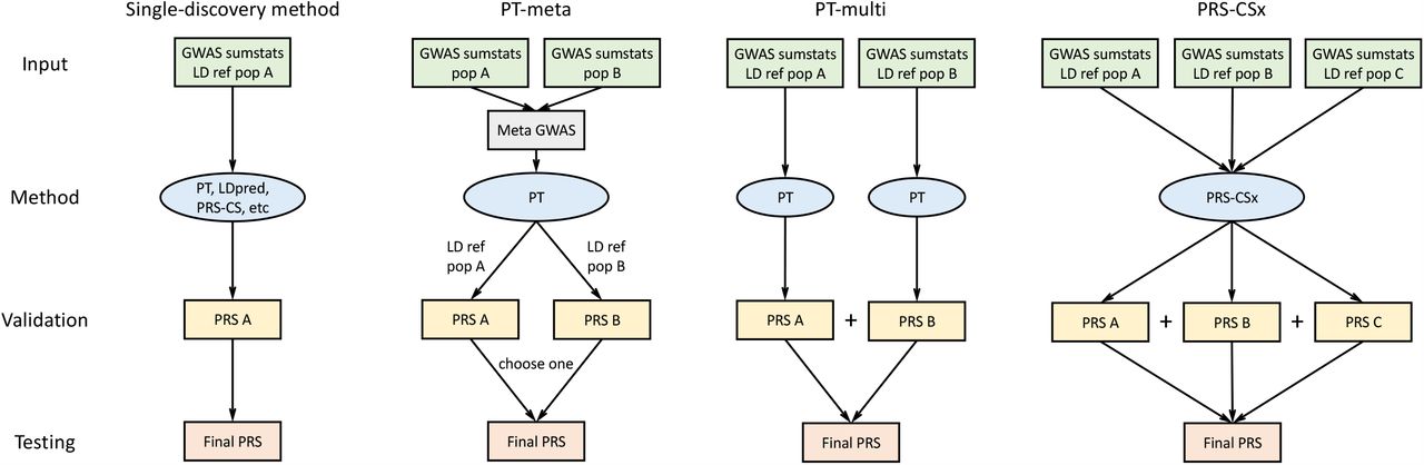
The discovery samples (to generate GWAS summary statistics), validation samples (to turn hyper-parameters of PRS construction methods) and testing samples (to assess prediction accuracy) are non-overlapping. LD ref: LD reference panel; pop A/B/C: Population A/B/C.
Overview of PRS analysis
We have broadly classified polygenic prediction methods into two categories: single-discovery methods, which train PRS using GWAS summary statistics from a single discovery sample; and multi-discovery methods, which combines GWAS summary statistics from multiple discovery samples for PRS construction. In this work, we assess and compare within- and cross-population predictive performance of three representative single-discovery methods: (i) LD-informed pruning and p-value thresholding (PT)29; (ii) LDpred22; (iii) PRS-CS24; and two multi-discovery methods in addition to PRS-CSx: (i) PT-meta, which applies PT to the meta-analyzed discovery GWAS summary statistics; (ii) PT-multi21, which applies PT to each discovery GWAS separately, and linearly combines the resulting PRS. This method has been demonstrated to improve the prediction in recently admixed populations. The workflow for each PRS construction method is shown in Fig. 1. In all the PRS analyses, we use the discovery dataset to estimate the marginal effect sizes of SNPs in each population and generate GWAS summary statistics; we use the validation dataset, with individual-level genotypes and phenotypes, to tune hyper-parameters for different polygenic prediction methods; and we use the testing dataset, with individual-level genotypes and phenotypes, to evaluate the prediction accuracy of PRS and compute performance metrics using hyper-parameters learnt in the validation dataset. The three datasets comprise non-overlapping individuals. For convenience, we use the target dataset to refer to the combination of validation and testing datasets, which have matched ancestry. For fair comparison across methods, we use 1000 Genomes Project (1KG) Phase 330 super-population samples (European N=503; East Asian N=504; African N=661) as the LD reference panels throughout the paper.
Simulations
We first evaluated the predictive performance of different PRS construction methods using simulations. We simulated individual-level genotypes of European (EUR), East Asian (EAS), and African (AFR) populations for HapMap3 variants with minor allele frequency (MAF) >1% in at least one of the populations using HAPGEN231 and the 1KG Phase 3 samples as the reference panel. We simulated a wide range of genetic architectures by randomly sampling 0.1%, 1% or 10% of the variants across the genome as causal variants, which in aggregation explained 50% of phenotypic variation. We assumed that causal variants are shared across populations but allowed for varying effect sizes, which were sampled from a multivariate normal distribution with the cross-population genetic correlation (rg) set to 0.4, 0.7 or 1.0. For each combination of the causal variant proportion (0.1%, 1% and 10%) and genetic correlation (0.4, 0.7 and 1.0), the simulation of the phenotype was repeated for 20 times.
We applied single-discovery methods (PT, LDpred, PRS-CS) to GWAS summary statistics generated by 20K, 50K or 80K simulated EUR samples and evaluated their predictive performance, measured by the squared correlation (R2) between the simulated and predicted phenotypes, in 20K EUR, EAS and AFR target samples, which were evenly split into a validation dataset (for hyper-parameter tuning) and a testing dataset (for the calculation of prediction accuracy) (Fig. 2; Supplementary Table 1). Consistent with previous observations7, all the three single-discovery methods had decreased prediction accuracy when the genetic distance between the discovery and target populations increases32, even if the causal variants and their effect sizes were identical between populations (i.e., rg=1.0). As expected, the prediction accuracy decreased further when genetic effects were less correlated across populations (rg=0.4 or 0.7), making effect size estimates less transferable. We also noted that, for a fixed heritability, the predictive performance of all single-discovery methods reduced as the genetic architecture became more polygenic, as measured by the proportion of causal variants, due to the increasing difficulty of accurately estimating small genetic effects and separating signals from noise. Among the three single-discovery methods examined, Bayesian methods (LDpred and PRS-CS) often outperformed PT, especially for polygenic architectures (1% or 10% causal variants). PRS-CS outperformed LDpred in both within- and cross-population prediction across different simulation settings with well-powered discovery GWAS (N=80K; Fig. 2), but may be less accurate than LDpred when the genetic architecture is highly polygenic (10% causal variants) and the discovery sample size is limited (N=20K or 50K; Supplementary Table 1).

Different genetic architectures (0.1%, 1% and 10% causal variants) and cross-population genetic correlations (0.4, 0.7 and 1.0) were simulated. Heritability was fixed at 50%. 80K simulated EUR samples were used as the discovery dataset for single-discovery methods. 20K samples from the target population (EAS or AFR) were added to the discovery dataset for multi-discovery methods. Prediction accuracy was measured by the squared correlation (R2) between the simulated and predicted phenotypes in the testing dataset, averaged across 20 simulation replicates. Error bar indicates the standard deviation of R2 across simulation replicates.
We then assessed whether multi-discovery methods (PT-meta, PT-multi, PRS-CSx) can improve cross-population polygenic prediction. Specifically, we added 20K simulated samples of EAS and AFR, respectively, to 20K, 50K or 80K EUR samples as the discovery dataset, and used different multi-discovery methods to combine GWAS summary statistics from two populations (EUR+EAS or EUR+AFR). Predictive performance was evaluated in 20K independent EAS or AFR target samples (Fig. 2; Supplementary Table 2). Similar to single-discovery methods, the predictive performance of multi-discovery methods decayed with increasing genetic divergence between discovery and target samples, decreasing concordance of SNP effect sizes measured by cross-population genetic correlation, and increasing polygenicity of the genetic architecture. In most scenarios, multi-discovery methods improved prediction accuracy over single-discovery methods, reflecting the increase in discovery sample size. Overall, PT-meta worked better when SNP effect sizes are highly concordant across populations (e.g., rg=1.0), justifying the use of a fixed-effect meta-analysis approach to combine summary statistics, while PT-multi outperformed PT-meta when cross-population genetic correlation is moderate (e.g., rg=0.4). PRS-CSx substantially improved cross-population prediction accuracy relative to alternative methods across all simulation settings (Fig. 2; Supplementary Table 2).
Prediction of quantitative traits in Biobanks
Next, we evaluated the predictive performance of different polygenic prediction methods using 17 anthropometric or blood panel traits – same as those used in Martin et al.7 – from UKBB25 (N=340,159-360,388) and BBJ26 (N=62,076-159,095; Supplementary Table 3). Summary statistics were acquired from the Neale Lab (UKBB GWAS) and BBJ website (Data availability). We removed basophil count due to its highly skewed distribution in UKBB, unmatched phenotypic transformations in the UKBB (untransformed) and BBJ (inverse rank normalized) GWAS, and the low genetic-effect correlations (ρge=0.35) between UKBB and BBJ, estimated by POPCORN16, leaving 16 quantitative traits for PRS analysis. All the 16 traits had matched phenotype scales, and had moderate to high cross-population genetic-effect correlations (minimum ρge=0.63; Supplementary Table 3). We applied single-discovery methods to UKBB or BBJ summary statistics, and used multi-discovery methods to combine UKBB and BBJ GWAS. All target samples are UKBB individuals that are unrelated with the UKBB discovery samples. We assigned each target sample to one of the five 1KG super-populations [AFR, AMR (Admixed American), EAS, EUR, SAS (South Asian)] using 1KG samples as the reference (see Methods), and assessed the prediction accuracy in each target population separately, adjusting for age, sex, age2, age x sex, age2 x sex, and top 20 principal components (PCs). For each population, the target samples were randomly and evenly split into a validation dataset (for hyper-parameter tuning) and a testing dataset (for the evaluation of predictive performance). The prediction accuracy, measured by variance explained (R2) in linear regression after accounting for covariates, was averaged across 100 random splits.
Consistent with simulation results, PRS-CSx outperformed alternative methods in almost all predictions examined when trained using UKBB and BBJ summary statistics (Fig. 3a; Supplementary Fig. 1; Supplementary Table 4). However, the improvement in prediction accuracy relative to PRS-CS trained on UKBB summary statistics, which is often the second best method, depended on the target population. When predicting into EUR, PRS-CSx provided a consistent but marginal improvement over PRS-CS (median increase in R2: 3.5%), likely because UKBB GWAS were already well-powered and thus adding a smaller non-European GWAS did not provide much additional information. When the target population is EAS, however, PRS-CSx substantially increased prediction accuracy relative to single-discovery PRS-CS: the median improvement in R2 was 18% when compared with PRS-CS trained on UKBB GWAS, and 76% when compared with PRS-CS trained on BBJ GWAS, suggesting that PRS-CSx can leverage large-scale European GWAS to improve the prediction in non-European populations. When the target population did not match any of the discovery samples, the benefits of integrating UKBB and BBJ GWAS appeared to be limited. For example, the median improvement of the prediction accuracy in AFR was 6.8%, but remained low relative to the predictions in EUR and EAS (Supplementary Fig. 1), likely because both discovery samples are genetically distant.

(a) Relative prediction accuracy of single-discovery and multi-discovery polygenic prediction methods, with respect to PRS-CS trained using UKBB GWAS, across 16 traits in different target populations (EUR, EAS and AFR). (b) Relative prediction accuracy of PRS-CS and PRS-CSx, with respect to PRS-CS trained using UKBB GWAS, across 7 traits in different target populations (EUR, EAS and AFR). Each point shows the relative prediction R2 of a trait, averaged across 100 random splits of the target samples into validation and testing datasets. Crossbar indicates the median of relative R2 across traits.
We then investigated whether adding AFR samples to the discovery dataset can improve the prediction in the AFR population. Among the 16 traits we examined, 7 were also available in PAGE27 (N=19,803-49,796), a genetic epidemiology study comprising largely of African American and Hispanic/Latino samples (Supplementary Table 3). Most UKBB-PAGE and BBJ-PAGE genetic-effect correlations were moderate to high (minimum ρge=0.60) except for mean corpuscular hemoglobin concentration (BBJ-PAGE ρge=0.38), which has the smallest GWAS sample size in PAGE (N<20K; Supplementary Table 3). Although the discovery and target samples had matched ancestry, applying PRS-CS to PAGE summary statistics alone produced low prediction accuracy in the AFR population due to sample size limitations of the PAGE study (Fig. 3b; Supplementary Fig. 1; Supplementary Table 4). However, integrating UKBB, BBJ and PAGE summary statistics using PRS-CSx dramatically outperformed single-discovery methods, and the median improvement in R2 was 22% (range: 21%-209%) compared with PRS-CSx trained on UKBB and BBJ GWAS only, suggesting that PRS-CSx benefits from including samples that have matched ancestry with the target population in the discovery dataset, even if the non-European GWAS included are considerably smaller than European studies. Adding PAGE as a discovery dataset for PRS-CSx in addition to UKBB and BBJ also consistently improved prediction accuracy in other target populations, although to a less extent (Figure 3b; Supplementary Fig. 1; Supplementary Table 4).
Schizophrenia risk prediction
Lastly, we evaluated the predictive performance of different polygenic prediction methods for dichotomous traits. We used schizophrenia as an example, for which large-scale EUR and EAS samples are available (Supplementary Table 5). Specifically, we used GWAS summary statistics derived from Psychiatric Genomics Consortium (PGC) wave 2 EUR samples (33,640 cases and 43,456 controls)28 and 10 PGC EAS cohorts15 (7,856 cases and 11,562 controls) as the discovery dataset. For the additional 7 EAS cohorts which we had access to individual-level data, we set aside one cohort (687 cases and 492 controls) as the validation dataset, and applied a leave-one-out approach to the remaining 6 cohorts. More specifically, we in turn used one of the 6 cohorts as the testing dataset, and meta-analyzed the remaining 5 cohorts with the 10 PGC EAS cohorts using an inverse-variance-weighted meta-analysis to generate the discovery GWAS summary statistics for the EAS population. The prediction accuracy of different PRS construction methods was then evaluated in the left-out (testing) cohort, adjusting for sex and top 20 PCs. As a reference, the SNP heritability of schizophrenia on the liability scale was estimated to be 0.23±0.03 in the East Asian population15.
Consistent with previous observations, PRS trained on EAS summary statistics were more predictive in EAS cohorts than those trained on PGC EUR summary statistics15, despite the larger sample size for the EUR GWAS (Fig. 4a; Supplementary Table 6). Bayesian methods (LDpred and PRS-CS) performed substantially better than PT, highlighting the importance of modeling LD patterns for highly polygenic traits. By integrating EUR and EAS summary statistics, PRS-CSx dramatically increased the prediction accuracy relative to single-discovery methods: the median R2 on the liability scale, assuming 1% of disease prevalence, increased from 0.040 (PRS-CS trained on EAS GWAS) and 0.031 (PRS-CS trained on EUR GWAS) to 0.060, a relative increase of 52% and 97%, respectively. PRS-CSx also approximately doubled the prediction accuracy of alternative multi-discovery methods, PT-meta and PT-multi, with a relative increase of 126% (from 0.027 to 0.060) and 88% (from 0.032 to 0.060), respectively, in the median liability R2 (Fig. 4a). Other performance metrics, including Nagelkerke R2, odds ratio (OR) per standard deviation change of PRS, and OR comparing top 10% with bottom 10% of the PRS distribution, showed a consistent pattern (Supplementary Table 6). Finally, PRS-CSx can more accurately identify individuals at high/low schizophrenia risk than alternative methods, showing a 2.9, 3.5 and 4.2 fold increase in case prevalence across the 6 testing cohorts when contrasting the top 10%, 5% and 2% of the PRS distribution with the bottom 10%, 5% and 2%, respectively (Fig. 4b; Supplementary Table 7).
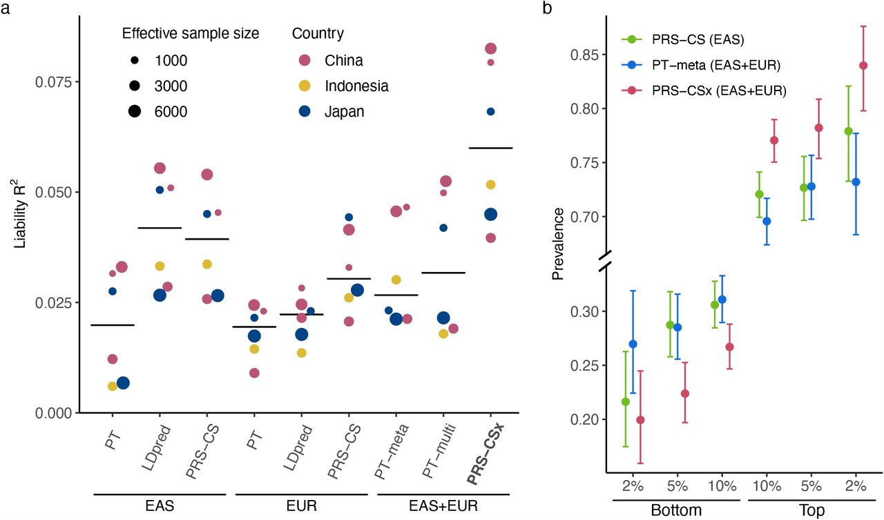
(a) Prediction accuracy, measured as R2 on the liability scale, of single-discovery (trained with EAS or EUR GWAS) and multi-discovery polygenic prediction methods (trained with both EAS and EUR GWAS: EAS+EUR) across 6 EAS schizophrenia cohorts. Each dot represents one testing cohort, with the size of the dot proportional to the effective sample size, calculated as 4(1/Ncase+1/Ncontrol). Crossbar indicates the median R2 on the liability scale. (b) Case prevalence of the bottom 2%, 5%, 10% and top 2%, 5%, 10% of the PRS distribution, constructed by PRS-CS, PT-meta and PRS-CSx. Error bar indicates 95% confidence intervals.
DISCUSSION
We have presented PRS-CSx, a Bayesian polygenic prediction method that integrates GWAS summary statistics from multiple populations to improve the prediction accuracy of PRS in ancestrally diverse samples. PRS-CSx leverages the correlation of genetic effects and LD diversity across populations to more accurately localize association signals and increase the effective sample size of the discovery dataset, while accounting for population-specific allele frequency and LD patterns. We have shown, via simulation studies, that PRS-CSx robustly improves cross-population prediction over existing methods across traits with varying genetic architectures, genetic correlations between populations, and discovery GWAS sample sizes (Fig. 2). Using quantitative traits from global biobanks (Fig. 3) and schizophrenia cohort studies of European and East Asian ancestries (Fig. 4), we have further demonstrated the PRS-CSx can leverage large-scale European GWAS to boost the accuracy of polygenic prediction in non-European populations, for which ancestry-matched discovery GWAS may be orders of magnitude smaller in sample size.
PRS-CSx appears to be most effective when one of the discovery samples has matched ancestry with the target population. Although PRS-CSx can take an arbitrary number of GWAS summary statistics as input, an ancestry-matched LD reference panel is required for each discovery sample, which may be challenging to build for GWAS conducted in admixed populations or in samples with large genomic diversity. For example, in this work, we have used an African reference panel to approximate the LD patterns in the PAGE GWAS, which largely comprised of African American and Hispanic/Latino samples27. Although we have shown that this approach improved the prediction in both African and admixed American populations, indicating that PRS-CSx is robust to imperfectly matched LD reference panels, future work is needed to better model summary statistics from recently admixed populations. One promising direction is to characterize and incorporate local ancestries in PRS construction using ancestry-specific effect size estimates33,34. The Bayesian modeling framework of PRS-CSx and the flexibility of continuous shrinkage priors also allow for the incorporation of functional annotations and fine-mapping results into PRS construction to improve the portability of PRS, as shown by recent studies35. Moreover, given that many diseases, such as autoimmune diseases and psychiatric disorders, have substantial genetic overlap, extending the PRS-CSx framework to integrate genetically correlated traits may further inform the construction of PRS and increase its prediction accuracy36.
Lastly, we note that although PRS-CSx can greatly improve cross-population polygenic prediction, the gap in prediction accuracy between European and non-European populations remains considerable. In fact, sophisticated statistical and computational methods alone will not be able to overcome the current Eurocentric biases in GWAS. Broadening the sample diversity in genomic research to fully characterize the genetic architecture and understand the genetic and non-genetic contributions to human complex traits and diseases across global populations is crucial to further improve the prediction accuracy of PRS in diverse populations. We believe that the rapid expansion of genomic resources for non-European populations coupled with advanced analytic methods will accelerate the equitable deployment of PRS in clinical settings and maximize its healthcare potential.
Data Availability
Publicly available data were downloaded from the following databases: 1000 Genomes Phase 3 reference panels: https://mathgen.stats.ox.ac.uk/impute/1000GP_Phase3.html; Genetic map for each subpopulation: ftp.1000genomes.ebi.ac.uk/vol1/ftp/technical/working/20130507_omni_recombination_rates; UKBB summary statistics: http://www.nealelab.is/uk-biobank (GWAS round 2 was used in this study); BBJ summary statistics: http://jenger.riken.jp/en/result; PAGE summary statistics were downloaded from the GWAS Catalog: https://www.ebi.ac.uk/gwas/downloads/summary-statistics; PGC wave 2 schizophrenia EUR GWAS (49 EUR samples): https://www.med.unc.edu/pgc/download-results/scz; Schizophrenia EAS summary statistics are available upon request to PGC Schizophrenia Work Group. Schizophrenia individual-level data of East Asian ancestry are available upon reasonable request with regulatory/compliance review to the Stanley Global Asia Initiatives: zguo@broadinstitute.org.
AUTHOR CONTRIBUTIONS
H.H. and T.G. designed the project; T.G. developed the statistical methods and programmed the code for PRS-CSx; Y.R. and T.G. conducted simulation studies; Y.R. completed the major part of real data analysis; Y.A.F. assigned the UKBB samples into super-population groups; C.C. provided critical suggestions for the study design; M.L. took part in the testing of the code and processed schizophrenia East Asian data; A.S. and S.Q. took a lead role in the generation and processing of schizophrenia East Asian data. Y.R., H.H. and T.G wrote the manuscript; A.R.M. provided critical revision for the manuscript; All the authors reviewed and approved the final version of the manuscript.
COMPETING INTERESTS
The authors declare no competing interests.
DATA AVAILABILITY
Publicly available data were downloaded from the following databases: 1000 Genomes Phase 3 reference panels: https://mathgen.stats.ox.ac.uk/impute/1000GP_Phase3.html; Genetic map for each subpopulation: ftp.1000genomes.ebi.ac.uk/vol1/ftp/technical/working/20130507_omni_recombination_rates; UKBB summary statistics: http://www.nealelab.is/uk-biobank (“GWAS round 2” was used in this study); BBJ summary statistics: http://jenger.riken.jp/en/result; PAGE summary statistics were downloaded from the GWAS Catalog: https://www.ebi.ac.uk/gwas/downloads/summary-statistics; PGC wave 2 schizophrenia EUR GWAS (49 EUR samples): https://www.med.unc.edu/pgc/download-results/scz; Schizophrenia EAS summary statistics are available upon request to PGC Schizophrenia Work Group. Schizophrenia individual-level data of East Asian ancestry are available upon reasonable request with regulatory/compliance review to the Stanley Global Asia Initiatives: zguo@broadinstitute.org.
CODE AVAILABILITY
The code used in this study is available from the following websites: PRS-CSx: https://github.com/getian107/PRScsx; PRS-CS: https://github.com/getian107/PRScs; LDpred: https://github.com/bvilhjal/ldpred; PRSice2: https://www.prsice.info; POPCORN: https://github.com/brielin/Popcorn; Interpolation of genetic maps: https://github.com/joepickrell/1000-genomes-genetic-maps; Population assignment: https://github.com/Annefeng/PBK-QC-pipeline; Analysis scripts: https://github.com/YunfengRuan/PRS_methods.
METHODS
PRS-CSx
PRS-CSx is an extension of PRS-CS24, which enables the integration of GWAS summary statistics from multiple populations to improve cross-population polygenic prediction. Consider the following Bayesian linear regression for K populations:
 where, for each population k, yk is a vector of standardized phenotypes (zero mean and unit variance) from Nk individuals, Xk is an Nk×Mk matrix of standardized genotypes (each column has zero mean and unit variance), βk is a vector of SNP effect sizes, ϵk is a vector of normally distributed non-genetic effects with variance
  , for which we assign a non-informative scale-invariant Jeffreys prior, I is an identify matrix. We place a continuous shrinkage prior on the SNP effect size, which can be represented as global-local scale mixtures of normals:
 where ϕ is a global shrinkage parameter shared across all SNPs that models the overall sparseness of the genetic architecture, and ψj is a local, SNP-specific shrinkage parameter that is adaptive to marginal GWAS associations. By assigning a gamma-gamma hierarchical prior on ψj (specifically, the Strawderman-Berger prior with a = 1 and b = 1/2 in this work), the marginal prior density of βjk has sizable amount of mass near zero to impose strong shrinkage on small noisy signals, and in the meantime, heavy Cauchy-like tails to avoid over-shrinkage of truly non-zero effects. We note that when a SNP is available in multiple populations, the continuous shrinkage prior is coupled across populations, enabling information sharing between summary statistics while allowing for varying SNP effect sizes across populations to retain modeling flexibility.
Given the summary statistics and ancestry-matched LD reference panel for each discovery sample, the PRS-CSx model can be fitted using a Gibbs sampler with block update of posterior SNP effect sizes, without the need to access individual-level data (Supplementary Methods). PRS-CSx inherits many features from PRS-CS, including robustness to varying genetic architectures, accurate multivariate modeling of population-specific LD patterns, and computational efficiency. In this work, we used pre-calculated 1KG Phase 3 LD reference panels37 for EUR, EAS and AFR, which were constructed for HapMap3 variants with MAF >0.01. We used 1,000 Markov Chain Monte Carlo (MCMC) iterations with the first 500 steps as burin-in in Gibbs sampling. The computation on the longest chromosome can be completed within about 2.5 hours. For a fixed global shrinkage parameter ϕ, PRS-CSx returns posterior SNP effect size estimates for each discovery population, which can be used to calculate PRS in the target dataset. For each ϕ value among 10−6, 10−4, 10−2 and 1.0, we learnt a linear combination of the standardized PRS (one for each discovery population) in the validation dataset. The optimal ϕ and the weights for the linear combination of PRS that maximized the R2 were used in the independent testing dataset to calculate the final PRS and its performance metrics.
Existing PRS methods
PT
LD-informed pruning and p-value thresholding (PT)29 selects clumped SNPs of a certain statistical significance to be included in the PRS calculation. We performed PT using PRSice-238 with the default parameter settings: the clumping was performed with a radius of 250kb and an r2 threshold of 0.1. We used 1KG super-population samples (EUR, EAS or AFR) whose ancestry matched the discovery sample as the LD reference panel for clumping. The p-value threshold among 10−8, 10−7, 10−6, 10−5, 3×10⁻⁵, 10−4, 3×10⁻⁴, 0.001, 0.003, 0.01, 0.03, 0.1, 0.3 and 1.0 that maximized the R2 in the validation dataset was selected, and used in the independent testing dataset to calculate the final PRS and its performance metrics.
Ldpred
LDpred22 is a Bayesian polygenic prediction method that adjusts marginal SNP effect size estimates from GWAS summary statistics to calculate the PRS. LDpred assigns a point-normal prior to SNP effect sizes, where the proportion of causal variants is a tunable parameter, and infers posterior effects using a Gibbs sampler. We constrained the computation to HapMap3 variants with minor allele frequency (MAF) >0.01, and used 1KG super-population samples (EUR, EAS or AFR) whose ancestry matched the discovery sample as the LD reference panel. We used default parameter settings and set the radius for local LD approximation to 400 following the recommendation of LDpred (∼1.2M HapMap3 variants divided by 3000). The proportion of causal variants among 10−5, 3×10⁻⁵, 10−4, 3×10⁻⁴, 0.001, 0.003, 0.01, 0.03, 0.1, 0.3 and 1.0 that maximized the R2 in the validation dataset was selected, and used in the independent testing dataset to calculate the final PRS and its performance metrics.
PRS-CS
PRS-CS24 is a Bayesian polygenic prediction method that infers posterior SNP effect sizes from summary statistics using a continuous shrinkage prior, which is robust to varying genetic architectures, accurate in LD modeling and computationally efficient. PRS-CS has one hyper-parameter, the global shrinkage parameter, which models the overall sparseness of the genetic architecture. We used default parameter settings and the pre-calculated 1KG LD reference panel (EUR, EAS or AFR) that matched the ancestry of the discovery sample, which was constructed for HapMap3 variants with MAF >0.01. The global shrinkage parameter among 10−6, 10−4, 10−2 and 1.0 that maximized the R2 in the validation dataset was selected, and used in the independent testing dataset to calculate the final PRS and its performance metrics.
PT-meta
PT-meta applies PT to the meta-GWAS that combine all discovery summary statistics through an inverse-variance-weighted fixed-effect meta-analysis. We used the same clumping parameters and screened the same list of p-value thresholds as the PT method. The 1KG LD reference panel (EUR, EAS or AFR) that had matched ancestry with each of the discovery samples was in turn used for clumping, producing multiple sets of clumped variants. The best combination of the LD reference panel and the p-value threshold that maximized the R2 in the validation dataset was selected, and used in the independent testing dataset to calculate the final PRS and its performance metrics.
PT-multi
PT-multi21 applies PT to each discovery summary statistics separately, and linearly combines the most predictive PRS derived from each discovery sample. We used the same clumping parameters and screened the same list of p-value thresholds as the PT method. The 1KG super-population samples (EUR, EAS or AFR) whose ancestry matched the discovery sample were used as the LD reference panel for clumping. The optimal p-value threshold for each discovery sample and the weights for the linear combination of standardized PRS that maximized the R2 were learnt in the validation dataset, and used the independent testing dataset to calculate the final PRS and its performance metrics.
Simulations
Genotypes:We simulated individual-level genotypes of EUR, EAS and AFR populations using HAPGEN231 and the 1KG Phase 330 samples as the reference panel. We grouped CEU, IBS, FIN, GBR and TSI into the EUR super-population, CDX, CHB, CHS, JPT and KHV into the EAS super-population, and ACB, ASW, LWK, MKK and YRI into the AFR super-population. To calculate the genetic map for each super-population, we downloaded the genetic maps for their constituent subpopulations (Data availability), interpolated the recombination rate at each map position (Code availability), and averaged the recombination rates across the subpopulations within each super-population. We simulated 80,000 samples for EUR, 20,000 samples for EAS and 20,000 samples for AFR as the discovery dataset. We additionally simulated 20,000 samples for each of the three populations as the target dataset, which was evenly split into validation and testing samples. We constrained the simulations to HapMap3 variants with MAF >0.01 in at least one of the EUR, EAS and AFR populations, and removed triallelic and strand ambiguous variants. Phenotypes: We randomly sampled 0.1%, 1% or 10% of the variants as causal variants. We assumed that causal variants are shared across the three populations and simulated their effect sizes using a multivariate normal distribution with the correlation between the European and non-European populations set to 0.4, 0.7 or 1.0. For each population, we used a normally distributed random variable to model the non-genetic component such that the heritability was fixed at 50%. We simulated 20 replicates for each combination of the causal variant proportion (0.1%, 1% and 10%) and cross-population genetic correlation (0.4, 0.7 and 1.0), producing a total of 540 simulated phenotypes. GWAS was performed on the discovery dataset using PLINK 1.939 for each simulated phenotype to generate summary statistics.
UKBB, BBJ and PAGE analysis
Discovery data: We downloaded GWAS summary statistics from UKBB25, BBJ26 and PAGE27 (Data availability). We selected 16 quantitative traits that were available in both UKBB and BBJ, among which 7 were also available in PAGE (Supplementary Table 3). We chose the untransformed or inverse rank normalized version of the phenotype in UKBB that matched the transformation used in BBJ GWAS. We used 1KG EUR and EAS samples as the LD reference panel for UKBB and BBJ summary statistics, respectively, when constructing PRS. The PAGE study was largely comprised of African American and Hispanic/Latino samples, for which we used 1KG AFR samples as the LD reference panel as an approximation. Target data: All target samples are UKBB individuals that are non-overlapping with the samples used in the UKBB GWAS. To perform population assignment on the UKBB samples, we selected variants that are available in both 1KG and the UKBB genotyped dataset, and removed variants meeting one of the following criteria in 1KG: (i) strand ambiguous; (ii) located on sex chromosomes or in long-range LD regions (chr6: 25-35Mb; chr8: 7-13Mb); (iii) call rate <0.98; and (iv) MAF <0.05. We performed LD pruning on the remaining variants in 1KG using PLINK39 (--indep-pairwise 100 50 0.2), yielding 149,501 largely independent, high-quality common variants. We then conducted principal component (PC) analysis using these LD pruned SNPs in 1KG samples, and projected SNP loadings onto UKBB samples with scale appropriately adjusted. Using 1KG as the reference, we trained a random forest model to predict the 5 super-population labels (AFR, AMR, EAS, EUR, SAS) using the top 6 PCs, and applied the trained random forest classifier to UKBB samples to predict the genetic ancestry of each UKBB participant. We retained UKBB samples that can be assigned to one of the super-populations with a predicted probability >90%. For each predicted population in UKBB, we selected a set of unrelated individuals and performed sample-level quality control (QC) by removing individuals meeting one of the following criteria: (i) mismatch between self-reported and genetically inferred sex; (ii) missingness or heterozygosity outliers; and (iii) sex chromosome aneuploidy. For EUR samples, we further removed those that were included in the Neale Lab GWAS. Lastly, we performed variant-level QC on the UKBB imputed dataset for each target population by removing variants meeting one of the following criteria: (i) call rate <0.98; (ii) MAF <0.01; (iii) Hardy-Weinberg equilibrium test p-value <10−10; and (iv) imputation INFO score <0.8. The final target dataset included 7,507 AFR, 687 AMR, 2,181 EAS, 8,412 SAS and 14,085 EUR individuals.
Cross-population genetic correlation
We calculated the genetic correlation between UKBB, BBJ and PAGE using POPCORN16 with default parameters. POPCORN requires the LD score40 and cross-covariance score as the input. We used the pre-computed scores for EUR-EAS (available from the POPCORN website), and computed the scores for EUR-AFR and EAS-AFR using the ‘compute’ function provided by POPOCORN on 1KG Phase 3 samples.
Schizophrenia datasets
Schizophrenia data used in this study is summarized in Supplementary Table 5. PGC wave 2 schizophrenia GWAS summary statistics28 were used as the European discovery dataset. Except for one cohort (TMIM1), EAS samples used as discovery and target datasets were described in Lam et al.15 TMIM1 was recruited from multiple university hospitals and local hospitals in Japan. Patients were diagnosed according to the Diagnostic and Statistical Manual of Mental Disorders, 4th Edition (DSM-IV) with consensus from at least two experienced psychiatrists. All patients agreed to participate in the study and provided written informed consent. The study was approved by the institutional review boards of the Tokyo Metropolitan Institute of Medical Science and all affiliated institutions. DNA samples were genotyped on the Illumina Infinium Global Screening Array-24 v1.0 (GSA) BeadChip at the Broad Institute, using standard reagents and HTS workflow procedures for genotyping. GWAS QC and imputation were performed using Ricopili41 with default parameters. When used as a target cohort, SNPs were further filtered by imputation INFO score <0.9 and MAF <0.01.
SUPPLEMENTARY TABLES
Supplementary Table 1: Prediction accuracy of single-discovery polygenic prediction methods in simulations. PRS were trained using EUR GWAS with different sample sizes (20K, 50K, 80K) and assessed in different target populations (EUR, EAS, AFR) across different genetic architectures (0.1%, 1%, 10% causal variants) and cross-population genetic correlations (0.4, 0.7, 1.0).
Supplementary Table 2: Prediction accuracy of multi-discovery polygenic prediction methods in simulations. PRS were trained using combined EUR GWAS with different sample sizes (20K, 50K, 80K) and non-European GWAS with 20K samples and assessed in different non-European target populations (EAS, AFR) across different genetic architectures (0.1%, 1%, 10% causal variants) and cross-population genetic correlations (0.4, 0.7, 1.0). PRS-CS trained on EUR summary statistics was included for comparison.
Supplementary Table 3: Quantitative traits used in this study from UKBB, BBJ and PAGE, and their heritability and trans-ethnic genetic correlation estimates.
Supplementary Table 4: Prediction accuracy of single-discovery and multi-discovery polygenic prediction methods in different target populations across quantitative traits.
Supplementary Table 5: Information for the schizophrenia samples used in this study.
Supplementary Table 6: Prediction accuracy of single-discovery and multi-discovery polygenic prediction methods for schizophrenia risk across 6 EAS cohorts.
Supplementary Table 7: Prevalence of schizophrenia cases at the bottom 2%, 5%, 10% and top 2%, 5%, 10% of the PRS distribution across 6 EAS cohorts, constructed by different polygenic prediction methods.
ACKNOWLEDGEMENTS
We thank the Neale Lab and Biobank Japan (BBJ) for releasing the genome-wide association summary statistics from UK Biobank (UKBB) and BBJ. Individual-level genotypes for UKBB samples were obtained under application 32568. We thank the Psychiatric Genomics Consortium (PGC) for providing us with the GWAS summary statistics for schizophrenia. T.G. is supported by NIA K99/R00AG054573. H.H. acknowledges support from NIDDK K01DK114379, NIMH U01MH109539, Brain & Behavior Research Foundation Young Investigator Grant, the Zhengxu and Ying He Foundation, and the Stanley Center for Psychiatric Research. A.R.M. is supported by NIMH K99/R00MH117229.
Footnotes
↵* Email: chinsir{at}sjtu.edu.cn (S.Q.); hhuang{at}broadinstitute.org (H.H.); tge1{at}mgh.harvard.edu (T.G.)


