
Abstract
Although the COVID-19 disease burden is heterogeneous across space, the U.S. National Academies of Sciences, Engineering, and Medicine recommends an equitable spatial allocation of vaccines based, for example, on population size, in the interest of speed and workability. Utilizing economic–epidemiological modeling, we benchmark the performance of this ad hoc allocation rule by comparing it to the rule that minimizes the economic damages and expenditures over time, including a penalty cost representing the social costs of deviating from ad hoc allocations that favor speed and workability. Under different levels of vaccine scarcity and different demographic characteristics, we consider scenarios where length of immunity and compliance to travel restrictions vary, and consider the robustness of the rules when assumptions regarding these factors are incorrect. The benefits from deviating are especially high when immunity is permanent, when there is compliance to travel restrictions, when the supply of vaccine is low, and when there is heterogeneity in demographic characteristics. Interestingly, a lack of compliance to travel restrictions pushes the optimal allocations of vaccine towards the ad hoc and improves the relative robustness of the ad hoc rules, as the mixing of the populations reduces the spatial heterogeneity in disease burden.
JEL Classification C61, H12, H84, I18, Q54
1 Introduction
Now that several vaccines against coronavirus disease 2019 (COVID-19) have been developed, an ongoing question for policymakers around the globe is to determine how to allocate the limited supplies. Most of the scientific literature on allocation has focused on demographic considerations within one jurisdiction [1; 2; 3] or on a global scale [4; 5; 6; 7]. This prior work has made important contributions to the debate. A missing piece in the allocation question is how to divide up limited quantities across jurisdictions (e.g. state, counties) that might have different demographic and epidemiological characteristics. A report on the allocation of a COVID-19 vaccine by the U.S. National Academies of Sciences, Engineering, and Medicine (NASEM) [8] states that “[i]f the federal government were to provide states with an allotment of COVID-19 vaccine, in the interest of speed and workability, federal allocation to states could be conducted based on these jurisdictions’ population size.” Such a rule could also be deployed by states, provinces, or territories when deciding how to allocate within their boundaries.
In this paper, we explore the economic and epidemiological trade-offs associated with such a fixed ad hoc allocation rule by comparing it to the optimal rule conditional on the level of scarcity of the vaccine. Throughout this paper when we refer to the “ad hoc allocation,” what we mean is a rule of thumb that favors “speed and workability,” so we follow the U.S. NASEM [8] allocation recommendation based on the jurisdictions’ population size. The optimal rule we consider is assumed to be one that minimizes the economic costs from health-related damages, vaccine expenditures, and a workability cost imposed on the planner for deviating from the ad hoc rule.
In a world where two jurisdictions are identical in terms of population, the ad hoc rule would divide the limited supply equally between the jurisdictions. However, it is much more likely that two jurisdictions, even if equally sized, have heterogeneous levels of infections (e.g. in terms of cases) at the time a vaccine is licensed and starts to be administered. Based on prior literature on spatial-dynamics of disease management, heterogeneity in infection levels may lead to significant deviations between the optimal spatial allocation and the ad hoc rule (see [9] for example).
Mechanisms leading to heterogeneous infection include the timing of the outbreak, demographic characteristics of the population (e.g. age structure [10] and essential worker status [11]), and the implementation of and compliance with preventative interventions; see [12; 13] for more details on how SARS-CoV-2 (i.e. the virus that causes COVID-19) prevalence varies across space. While compliance to preventive measures may seem independent from vaccine allocation, it affects the initial conditions (i.e. the conditions before the vaccine is licensed and starts to be administered) and the conditions under which the limited supplies will be allocated. For example, compliance to shelter-in-place and travel restrictions results in little to no movement of the virus from one jurisdiction to another. When regions are non-interacting, Brandeau et al. [14] show for a general susceptible–infected–susceptible (SIS) model that the optimal allocation of resources depends on numerous intrinsic factors, including the size of the populations of each region and the initial level of infection. When regions are interacting, Rowthorn et al. [15] show when there is no immunity (i.e. in an SIS model) that treatment should be preferentially directed towards the region that has the lower level of infection. While these results indicate that a fixed ad hoc rule is less cost-effective in an SIS model, whether compliance to travel restrictions makes the ad hoc rule relatively more cost-effective in the case of COVID-19 is an open question.
Our findings illustrate that the vaccines should be optimally allocated over time depending on: (i) if the jurisdiction has initially a lower or higher disease burden, (ii) if immunity is permanent (see Zhou et al. [16]) or temporary (Gersovitz and Hammer [17] already pointed out that the optimal allocation is conditional on the duration of immunity), (iii) whether there is compliance to travel restrictions or not, (iv) the amount of vaccine available, and (v) the average demographic characteristics of the population (i.e. age structure and essential worker status). We proxy variability in demographics by assuming that the population of one jurisdiction has a higher case-fatality ratio (mimicking an older population) or a higher contact rate (mimicking a population containing more essential workers) than the other. We find that the benefits of deviating from the ad hoc rule are especially high when immunity is permanent, when there is compliance to travel restrictions, when the vaccine supply is low, and when there is heterogeneity in demographic characteristics. Allocating a vaccine based on an ad hoc allocation rule generally leads to an over-utilization in jurisdictions where disease prevalence is higher, an under-utilization in jurisdictions where disease prevalence is lower, and overall a higher number of cumulative cases. Whether these inefficiencies outweigh the “speed and workability” inherent in ad hoc rules is an important question for policymakers. Our research can aid in that discussion by illuminating the trade-offs involved in such complex epidemiological, economic, and social decisions by providing optimal benchmarks from which to compare ad hoc rules.
While the optimal allocation is conditional on a number of factors mentioned above, the science remains unresolved on the duration of immunity to SARS-CoV-2, and it is difficult to anticipate and subsequently estimate the extent to which populations in different jurisdictions comply with the travel restrictions. On the other hand, the ad hoc allocations have the advantage of being based on easily observable factors (e.g. a jurisdiction’s population size). To gain insights into the robustness of optimal and ad hoc policies in the presence of such uncertainties, we investigate the economic and public health consequences that could occur if we design an optimal policy or evaluate the performance of ad hoc rules under a set of assumptions on immunity and compliance that turn out to be incorrect.
We make a number of contributions to the literature. First, we develop an economic–epidemiological model and solve for the optimal allocation of vaccines over time to minimize the economic costs from damages, vaccine expenditures, and a workability cost imposed on the planner for deviating from the ad hoc rule. Prior literature considering the trade-offs involved with ad hoc rules does not consider that deviating from them entails potential workability costs (see, for example, [18]). Second, we consider how vaccine allocations are influenced by compliance with preventative interventions (i.e. travel restrictions). Third, we demonstrate how vaccine allocations are dependent on various demographics (i.e. age structure and essential worker status). Fourth, we show that, in general, optimal rules are robust to incorrect assumptions about the duration of immunity but differences in public health outcomes (cumulative cases) appear when compliance to a travel restrictions is assumed when in fact there is not compliance; it is, however, much preferable from a public health outcome perspective to comply with travel restrictions.
The paper is divided as follow. In Section 2, we detail the different types of interventions, we present the components of the economic-epidemiological model, and detail the technique used to analyse the allocation question. Section 3 presents the results while Section 4 concludes the paper.
2 Material and Methods
We develop an economic–epidemiological model to describe the dynamics of SARS-CoV-2. The model captures a situation where a central planning agency (e.g. the federal government) must decide when and how much of the scarce vaccines to allocate to two jurisdictions where disease burden is heterogeneous at the moment the vaccine is licensed and starts to be administered. We assume that the objective of the central planner is to minimize costs across both jurisdictions, including damages associated with the morbidity and deaths of infected individuals, the expenditures related to the pharmaceutical intervention, and a penalty cost mimicking the increased workability costs incurred for any deviation from the ad hoc allocation. The dynamics of SARS-CoV-2 are modeled using an SEIR epidemiological model, which tracks the change over time of the susceptible (S), exposed (E), infected (I), and recovered (R) populations for two separate jurisdictions (see Appendix A for more details on the calibration of the model). We note that while we generally talk about these jurisdictions as being two different states, they can very well represent two counties, or regions within one state.
2.1 Modelling Different Types of Intervention
There are two different types of interventions we consider: travel restrictions and vaccines. We assume that travel restrictions affect both jurisdictions simultaneously (e.g. by an order from the central government), and that the populations either comply perfectly or imperfectly to the travel restrictions (for examples of optimal lockdown policies see, e.g., [19; 20]). When compliance is perfect, individuals in different jurisdictions do not interact with each other and thus susceptible individuals can only get infected by being in contact with some infected individual in their own jurisdiction. When compliance is imperfect, susceptible individuals from one jurisdiction can also travel to the other jurisdiction where they can be in contact with infected individuals, or infected individuals from one jurisdiction can travel to the other jurisdiction and infect susceptible individuals there; this discrete shift in the number of contacts effectively increases the transmissibility of the virus (see Appendix A more details).
We assume that the analysis starts when a vaccine has already been developed, licensed, and is available in a relatively high quantity. For simplicity, the amount of available vaccine is assumed to be exogenous to the model and fixed over time, which is likely given the short time frames we consider in the paper. However, we consider different levels of vaccine supply to investigate how different levels of vaccine scarcity may affect their optimal allocation. In our model, vaccines reduce the pool of susceptible individuals by providing them with immunity from the virus, as early evidence suggests that vaccines could be transmission blocking in addition to preventing severe disease [21].
2.2 Model of Disease Transmission
We use a frequency-dependent [22] susceptible–exposed–infected–recovered (SEIR) model that describes the dynamics of COVID-19 in two separate jurisdictions i = 1, 2 (e.g. states/provinces or counties/administrative regions); each jurisdiction contains a population of Ni individuals that is either susceptible, exposed, infected, or recovered (see Figure 1). We also consider scenarios where immunity is temporary (i.e. lasts 6 months, for more details see [23]), thus also using an SEIR–Susceptible (SEIRS) model (for COVID-19 applications see, e.g., [24; 25; 26; 27; 28; 29; 30; 31; 32; 33; 34]). In such scenarios, the Ri recovered individuals are immune for a mean period of  months.

This schematic shows the model interventions and disease transmission pathways for our model of COVID-19. The full lines represent the transition between, or out of, compartments while the dotted lines represent contact between susceptible and infected individuals. Black lines represent situations that do not vary, while yellow lines represent key factors that we vary in our model to see how they impact our results. The green line represent the vaccines and the red line represents mortality.
In each jurisdiction i, the Si susceptible individuals are in contact with the Ii infected individuals of their own jurisdiction at a rate of βii and are in contact with the Ij infected individuals of the other jurisdiction at a rate of βij. We assume βij = 0 (i.e. no mixing between jurisdictions) when there is perfect compliance to travel restrictions, and βij > 0 if not. To highlight the role of travel restriction compliance and initial disease burden, we initially assume that the contact rate is identical across jurisdictions, meaning that β11 = β22 = βii and β12 = β21 = βij (in Section 3.2 we relax this assumption and investigate the optimal allocation when there is heterogeneity in the contact rate). We assume there is no permanent migration of individuals from one jurisdiction to another (see for instance [35] and see [36] for an example applied to COVID-19) in the sense that individuals who do not comply with travel restrictions do not permanently move to the other state, but instead travel to it temporarily. An implication is that we are assuming that the two jurisdictions are close enough for such travel and mixing to be economically feasible.
We model the control variables for vaccines as non-proportional controls, i.e. available in a constant amount each month [3; 15; 37; 38]. The change in susceptible individuals is
 where
where  represents the number of individuals being treated via vaccine in a given time period (i.e. a month) in Jurisdiction i, and qV represents the effectiveness of the vaccine. We note that our model does not distinguish between individuals whose vaccine has failed and those who have not been vaccinated at all. As such, individuals with vaccine failure can be re-vaccinated in subsequent months.
After being infected, susceptible individuals transition into the exposed class Ei where the disease remains latent for a mean period of time of  , before the onset of infectiousness. The change in the number of exposed individuals is
 Exposed individuals eventually become infectious for a mean period of time of
  and in turn can infect susceptible individuals. Infected individuals either recover naturally from the disease at a rate of γ or die from complications related to infection at a disease induced mortality rate of φi. In our base case we assume identical disease induced mortality rates across jurisdictions, i.e. φ1 = φ2 = φ but investigate the optimal allocation when φ1 = φ2 in Section 3.2. The growth of the infected individuals is
 The recovered population Ri includes individuals that recover naturally from the disease at a rate of γ and the individuals that are successfully vaccinated every month
  ; if immunity is temporary (ω > 0), a fraction of the recovered will leave this compartment. Our model does not distinguish between vaccine-acquired immunity and naturally-acquired immunity. The number of recovered individuals in Jurisdiction i thus changes according to
 At any instant in time, we have that Ni = Si + Ei + Ii + Ri, which in turn implies that the growth of the population over time is
 In keeping with much of the previous economic epidemiology literature [17] as well as recent applications to COVID-19 (see for example [39]), we have omitted natural births and non-COVID-related deaths due to the short time frame of our model (4 months) and assume reductions in international travel [40] effectively lead to a closed population (i.e. there is no exogenous importation of infected individuals). See Appendix A for more details about the parameterization of the epidemiological model.
2.3 Modelling Ad Hoc Allocations
We model an ad hoc allocation rule that favors “speed and workability” [8]. We follow the NASEM approach [8] and impose that the allocation is based on relative population sizes. Specifically, the rule for Jurisdiction i is that
 where
where  is the limited amount of vaccine available for both jurisdictions. When the population sizes are the same, the ad hoc rule will divide equally the limited doses to the two jurisdictions.
In the ad hoc scenarios, we model the allocation rule as an inequality because towards the end of the horizon after periods of vaccinations, the level of susceptible in the population may be such that the limited supply of vaccines is not an issue. Other ad hoc rules are possible, such as, allocate all to the largest or smallest population [18], but we concentrate on the one currently being advocated for by NASEM [8].
2.4 Model of Economic Costs
The model of economic costs include damages related to morbidity and deaths, costs spent on the vaccines, and the workability cost described above that is incurred for any deviation from the ad hoc allocation rule. Damages represent consequences related to a temporary disability associated with severe or critical symptoms, and loss of life in the worst cases. The damages are assumed to be linear and additively separable across jurisdictions, meaning that they are identical across individuals and across jurisdictions. The marginal value of damages (i.e. the damages associated with the death of one individual) is assumed to be constant over time and given by the value of a statistical life (VSL) that the U.S. Environmental Protection Agency [41] uses (see Appendix A for more details on the parameterization). Damages incurred from a temporary disability associated with severe or critical symptoms can be compared to deaths via some disability weight w; given the World Health Organization (WHO) has not yet published disability values associated with COVID-19, following the literature (see for instance [42]), we use the disability value associated with lower respiratory tract infections. The damage function for Jurisdiction i is
 where c is the damage parameter associated infectious individuals (i.e. the VSL).
We model a scenario where the central planner is focused on the allocation of vaccines where the costs for its development have already been incurred. This implies that vaccine development costs have already been utilized (in technical terms we say that the costs are sunk) and therefore do not affect the decision of the central planning agency. We model the vaccination cost as linear, where the cost parameter represents the cost of treating one individual. The vaccine cost function is denoted  , with i = 1, 2. We assume that the vaccination cost is additively separable across jurisdictions such that we denote the cost of treating
  individuals as
 where cV represents the cost of treating one individual via vaccine. Calibration of the cost parameter is based on current vaccine prices (see Appendix A for more details about the parameterization of the economic model).
We assume that the central planning agency incurs a workability cost representing the social (transaction) costs of deviating from the ad hoc allocation rule (for another application of this concept, see [43]). The workability cost function is:
 where cA is the parameter associated with the workability cost. When the gains from deviating from the ad hoc allocations (i.e. a reduction in damages in one jurisdiction) outweigh the costs (i.e. an increase in damages in the other jurisdiction and the increased workability costs incurred), the central planning agency will prioritize this allocation as it will lead to lower total costs. By imposing the ad hoc rule ex ante, the decision-maker is essentially assuming that this workability cost is infinite. Everything else being equal, we expect that the presence of the workability cost will push the optimal allocation towards the ad hoc rules (see Figure A18 for a sensitivity analysis of our results to the workability cost parameter). Therefore, when we do find deviations, we need to consider that these include this workability cost and if workability costs smaller, then the deviations and trade-offs would be greater.
2.5 Planner’s Objective
In optimal control theory, the best, or optimal, path of the control variables (here the allocation of the limited supply of vaccines) is conditional on the objective of the central planning agency. We assume that the objective is to minimize the economic damages and the costs of the pharmaceutical intervention across jurisdictions over time, rather than a solely epidemiological objective (see for instance [15]). The objective function is the net present value of damages, expenditures related to vaccination, and the workability cost over an exogenously determined planning horizon (4 months). Specifically, the planner’s objective is:
 where r is monthly discount rate. The planner solves equation (10) over a fixed time interval, T, subject to equations (1), (2), (3), (4), (5), along with constraints on availability of vaccines
  , non-negativity conditions, physical constraints on vaccines, initial disease burdens in each jurisdictions, and free endpoints (see discussion on terminal conditions in the next section). In the ad hoc scenarios, we also impose equation (6).
2.6 nitial and Terminal Conditions
The disease burden in each jurisdiction at the beginning of the time horizon (i.e. in t = 0 when the vaccine is already licensed and starts to be administered) is calibrated using the epidemiological model (equations (1), (2), (3), (4), and (5)). At the beginning of the outbreak, we assume that, in each jurisdiction, there is one exposed individual in an otherwise entirely susceptible population of 10 million individuals (approximately the population of Michigan), and that populations of the different jurisdictions comply with the travel restrictions. The only difference between the two jurisdictions is that the outbreak started one week earlier in State 2. We simulate the outbreak for approximately nine months to yield the initial conditions; see Appendix B for more details. In Section 3.2 when we consider heterogeneity in demographic characteristics (varying case-fatality ratio and contact rate), we modify the initial conditions accordingly assuming an identical timing in the outbreak of the disease.
We impose no conditions on the number of susceptible, exposed, infected, and recovered individuals at the end of the planning horizon; in technical terms, we say that the state variables are free (see Appendix B for more details). Under our free endpoint conditions, there is a transversality condition (i.e. a necessary condition for the vaccine allocation to be optimal) for each state variable that requires the product of the state variable (Si, Ei, Ii, Ri or Ni) and its corresponding costate variable (i.e. the shadow value, or cost, associated with the state variable) is equal to zero. Hence, at the end of the time horizon, either the state variable equals zero, the shadow value associated with the state variable equals zero, or both. In any case, allowing state variables to be free guarantees that the terminal levels of the state variables are optimally determined. Another possible assumption could be that over a fixed interval we find the optimal policy such that at the end of the horizon there is a given percent reduction in infected or susceptible individuals. Our approach nests this more restricted scenario.
3 Results
To examine the optimal allocations of vaccine over time, we numerically solve the optimal control problem across three different scenarios: no controls, optimal vaccine allocation, and ad hoc vaccine allocation. We investigate how to allocate vaccines by mapping out the different allocation rules for different immunity–travel restrictions–capacity scenarios. Any deviation from the ad hoc allocation rule is optimal despite incurring the workability cost. As the workability cost parameter cA goes to zero, the problem becomes linear in the controls where the optimal allocations in linear problems follow singular solutions. We use pseudospectral collocation to solve for the optimal dynamics of vaccine and infection over time, which converts the continuous time optimal control problem into a constrained non-linear programming problem solving for the coefficients of the approximating polynomials at the collocation nodes (see [44; 45] for other applications, and see Appendix B for more details on this technique).
We present the results for our preferred specification of the parameters (i.e. following what was estimated in the literature; see details in Appendix A) and for the case where immunity is permanent and the case where immunity is temporary. We detail the optimal deviation based on whether the populations of the different jurisdictions are compliant to travel restrictions or not, and for different levels of capacity constraints. The total available quantity of vaccine in a given time period (i.e. a month;  ) is based on a certain percentage (5%, 10%, or 15%) of the total population size. We focus our analysis on the period of time when the scarcity of the vaccine constraint is binding, as once the constraint relaxes the allocation question becomes moot.
3.1 Base Case: Homogeneous Demographic Characteristics
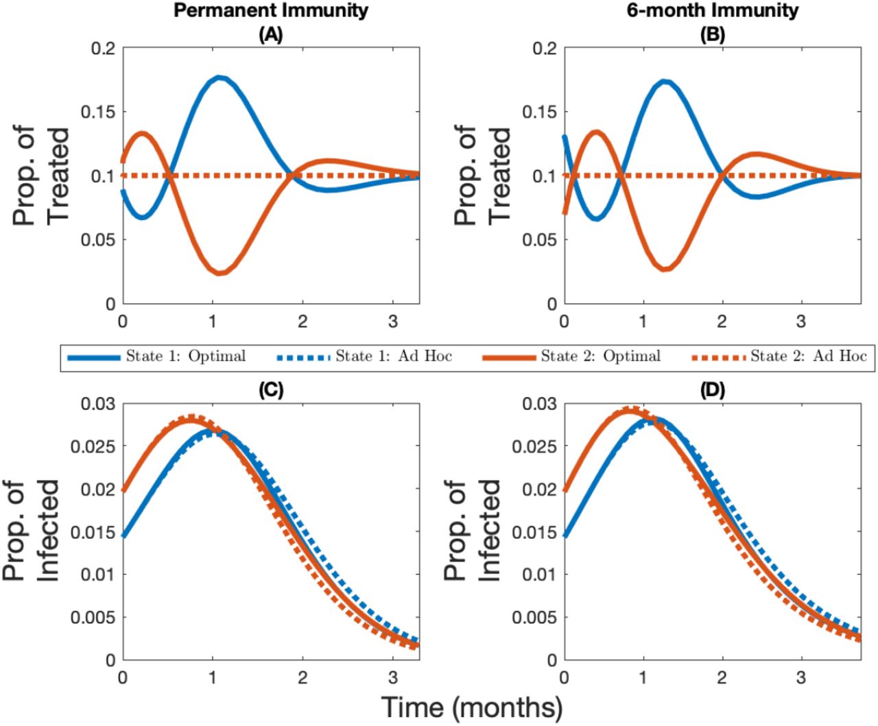
Compliance to travel restrictions impacts the optimal allocation of vaccines, regardless of whether immunity is temporary or permanent and regardless of the amount of vaccine available. Noncompliance to travel restrictions reduces both the oscillation (i.e. back-and-forth movement of resources between jurisdictions) of the optimal allocation and the amplitude of the deviations from the ad hoc rule (see Figure 2 for when immunity is permanent, and see Figure A1 for when immunity is temporary). Because noncompliance to travel restrictions decreases the structural heterogeneity in the system, the optimal allocation of vaccine converges towards the ad hoc allocation when populations mix with each other. This result clearly demonstrates how the performance of the allocation rule is dependent on how citizens in the jurisdictions comply with travel restrictions.

Change over time in the optimal and ad hoc allocations (panels A and B) and the corresponding infection levels (panels C and D) for State 1 (in blue, the initially lowest-burdened state) and State 2 (in red, the initially highest-burdened state) depending on whether there is compliance to travel restrictions (panels A and C) or not (panels B and D) for the case where the vaccine capacity constraint is 10% and immunity is permanent. Note the changing y-axis in panels C and D in order to better highlight the infection levels.
Noncompliance to travel restrictions leads to the initially less infected state being favored by the optimal allocation for low levels of vaccine capacity (e.g. 5% capacity; see Figure 3 Panel A for when immunity is permanent and Figure A4 Panel A for when immunity is temporary). On the other hand, the more infected state will be prioritized at the beginning of the time horizon for a very short period of time when vaccine capacity is larger (e.g. 10% or 15% capacity; see Figure 3 panels B and C for when immunity is permanent and Figure A4 panels B and C for when immunity is temporary). More generally, regardless of whether or not populations are compliant with travel restrictions, and regardless of whether immunity is temporary of permanent, a higher vaccine capacity implies that relatively more of the supply should be given to the more infected state at the beginning of the time horizon (see figures 3 and A2 for the case where immunity is permanent; see figures A3 and A4 for the case where immunity is temporary).
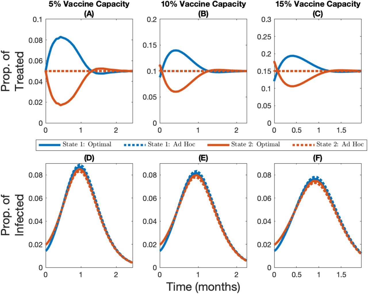
Change over time in the optimal and ad hoc allocations (panels A, B, and C) and the corresponding infection levels (panels D, E, and F) for State 1 (in blue, the initially lowest-burdened state) and State 2 (in red, the initially highest-burdened state) depending on whether capacity is 5% (panels A and D), 10% (panels B and E), or 15% (panels C and F), for the case where immunity is permanent and there is no compliance to travel restrictions.
Interestingly, temporary immunity has a different effect on the optimal vaccine allocation depending on whether or not populations are compliant to travel restrictions. When populations comply with travel restrictions, temporary immunity increases the oscillation of the optimal allocation because benefits from vaccination are only temporary, and since the population gradually loses its immunity, it forces more back-and-forth movement of resources between jurisdictions (see Figure A5). When populations do not comply with travel restrictions, temporary immunity reduces the amplitude of the deviations from the ad hoc rule because it further dampens the structural heterogeneity in the system, since the infection and recovery level of both jurisdictions will eventually reach the same positive steady-state level (recall the only heterogeneity in the system is the initial disease burden in the base case).
While the optimal allocation of vaccine is unequal from a resource allocation perspective, it equalizes the current infection levels across jurisdictions (Figure 2 Panel C). As the vaccine capacity increases, however, the ad hoc allocation rule performs better and in turn the amplitude of the optimal deviation decreases (see Figure A2 panels A, B and C, or Figure A3 panels A, B, and C). These optimal cost-minimizing deviations that lead to equal current infection levels across jurisdictions towards the end of the time horizon imply that the optimal cumulative number of cases is more unequal than in the ad hoc allocation (Figure 4). Hence, the optimal allocation makes the current infection level more equal, while the ad hoc allocation makes cumulative infection more equal. In fact, in all scenarios considered, the optimal allocation will lead to lower cumulative damages in the less infected jurisdiction but higher cumulative damages in the most infected jurisdiction (see Figure 4 with vaccine capacity of 10%, and see figures A7 and A8 with vaccine capacity of 5% and 15%, respectively).

Cumulative relative difference (panels A, B, C, and D) and cumulative absolute difference per 1M people (panels E, F, G, and H) between the number of infections in different allocations rules and the no-vaccine case for different immunity–travel restrictions scenarios and for when vaccine capacity is 10%.
3.2 Heterogeneous Demographic Characteristics
In our main analyses, we introduced heterogeneity in infection across jurisdictions by assuming a different timing in the outbreak of the virus. While this leads to heterogeneity in the disease burden, there are other mechanisms that could lead to similar differences in the disease burden at the time the vaccine is licensed and starts to be administered. For instance, in jurisdictions that have an older population on average, we expect SARS-Cov-2 to have a higher case-fatality ratio [10] which would effectively decrease the transmissibility of the virus (see Appendix A more details). If we assume that one jurisdiction has a higher case-fatality ratio and start the initial outbreak at the same time, then we find the population with the highest case-fatality ratio also has the largest population of susceptible individuals at the time the vaccine is administered. The heterogeneity in initial disease burden stems from the lower transmissibility in the jurisdiction with the higher case fatality ratio. The heterogeneity in case fatality ratio therefore not only leads to heterogeneity in the initial disease burden but it also implies that the benefits of vaccination are no longer homogeneous across jurisdictions. These differences lead the optimal allocation to favor even more the least burdened jurisdiction, which is also the most vulnerable (aka more older individuals) of the two populations. Overall, introducing heterogeneity in case fatality ratio strengthens our main set of results (see Figure A9 for when immunity is permanent and see Figure A10 for when immunity lasts 6 months).
Another source of heterogeneity in infection could stem from one jurisdiction having more essential workers than the other (for more details on how the risk of infection is occupation-dependent, see [11]). In our model, we can capture this by considering spatial heterogeneity in the contact rate, where a higher contact rate proxies for more essential workers. This in turn leads to a higher initial disease burden in the jurisdiction with higher contact rate. We find that priority is given to the state with a higher contact rate (aka more essential workers) in almost all cases. As the state with a higher contact rate gets vaccinated, we eventually shift priority to the state with the lowest contact rate because either the number of cases starts decreasing in the jurisdiction that has the higher contact rate, or the low-contact state eventually reaches a point where its infection level becomes higher than the high-contact state (see Figure A11 for when immunity permanent and see Figure A12 for when immunity lasts 6 months). In the case when immunity lasts 6 months and there is compliance to travel restrictions (Figure A12, Panel A), we find that priority is given to the low-contact jurisdiction, which contradicts many notions of fairness associated with vaccine allocation. With the gains of vaccination temporary and no movement of people, it turns out that the greatest return per vaccination is in the place where you can best avoid future cases (low contact rate jurisdiction). This prioritization is only fleeting however and there is more back-and-forth movement of resources between jurisdictions in this case, even though the workability cost is being incurred each time.
3.3 Robustness of Spatial Allocations
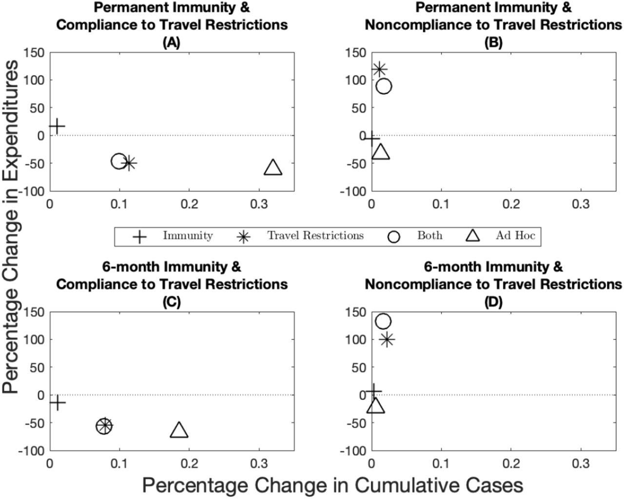
There is significant uncertainty associated with the duration of immunity (i.e. if it is permanent or temporary) and to what extent populations comply with travel restrictions. One argument for the ad hoc allocation is that uncertainty in these parameters makes the optimal allocation impossible to achieve. This uncertainty is not yet resolved and public health officials have to choose vaccine allocations based on potentially incorrect assumptions. We compare the robustness of the optimal spatial allocation to the ad hoc allocation. By definition, the optimal allocation minimizes the net present value of the health-related damages and total expenditures (including vaccine expenditures and the workability cost incurred because of the deviations from the ad hoc allocation), and thus cannot do worse on this dimension than the ad hoc allocation. We measure robustness by first inserting the optimal solution under one set of assumptions into the disease dynamics under another set and compute the changes in total expenditures (i.e. the pharmaceutical intervention and the workability cost) and public health outcomes (cumulative cases) over time. We then calculate the distance of these changes in percentage terms to the optimal solution derived under the “correct” assumptions (represented by the point (0, 0) in Figure 5). For example, suppose immunity is permanent and there is perfect compliance to a travel restriction. We derive the optimal policy under these assumptions and use it to measure the robustness of the optimal policies that are derived under assumptions that immunity is temporary and/or there is noncompliance. The ad hoc policies being based on observable factors are then compared to the incorrectly applied optimal policies. We illustrate the case for 10% scarcity and include other scarcity cases in Appendix C.

Percentage change in expenditures (y-axis) and percentage change in cumulative cases (x-axis) from the optimal allocation for different immunity–travel restrictions scenarios and for when vaccine capacity is 10%. The x-axis represent small percentage changes but when scaled up to population level effects translate into significant differences in public health outcomes.
When demographic characteristics are homogeneous across jurisdictions, we find overall that immunity length has a lesser impact on both economic and epidemiological outcomes than compliance to travel restrictions (compare the distance from the origin between the plusses and the stars in Figure 5). There are more nuanced trade-offs, however (e.g. compare position of the stars across the panels in Figure 5). Across the economic dimension (expenditures), for example, we find that assuming compliance when in fact there is very little leads to greater expenditures. Recall by design, the ad hoc allocations have lower expenditures than the optimal policies because the central planner is not incurring the workability costs from deviating off of the allocation. At the same time, greater cumulative cases result when the opposite holds, that is, assuming no compliance when in fact there is compliance. We also see that in some instances that the combined effect of incorrectly assuming the wrong immunity and compliance can offset some deviations (e.g. see Figure 5 Panel C) while in other cases the results are dominated by non-compliance. Finally, when there is compliance to travel restrictions the ad hoc allocation performs worse than any of the optimal allocations, while the ad hoc allocation performs relatively well when there is no compliance to travel restrictions. Varying the level of scarcity does not change the qualitative nature of results (see figures A13 and A14 for when vaccine capacity is 5% and 15% respectively), except for one anomaly where the ad hoc does not always perform worse under assumptions on compliance to travel restrictions (Figure A14).
We also investigate the robustness of the optimal allocations when the demographic characteristics are heterogeneous across jurisdictions. When jurisdictions have a different case-fatality ratio, the ad hoc allocation performs better than the optimal allocations when considering cases as the main health outcome (Figure A15). However, this approach is misleading because when case-fatality ratios are heterogeneous across jurisdictions, the cumulative aggregate number of cases (all jurisdictions together) is a poor outcome measure as a case in one place is not the same as a case in another jurisdiction. In this setting, the disease burden and cumulative damages give a more accurate depiction of the situation. In fact, while the ad hoc allocation outperforms the optimal allocations in terms of cumulative cases, it performs considerably more poorly when considering cumulative damages. We generally find that the optimal allocations outperform the ad hoc allocation in all scenarios considered (Figure A16). When jurisdictions have a different contact rate, the same pattern as in Figure 5 holds in the sense that when there is compliance to travel restrictions, the optimal allocations outperform the ad hoc allocation, while the ad hoc generally performs better than the optimal allocations when there is noncompliance to travel restrictions (Figure A17).
3.4 Sensitivity Analyses
The previous section considers the robustness of optimal allocations to incorrect assumptions about parameters (e.g. assuming permanent immunity while in fact it is temporary). Public health officials will also want to know how much optimal allocations change when parameters change (e.g. because vaccine effectiveness is lower against a new strain of the virus). We address those questions in this section. While both sets of analyses address parameter uncertainty, you can consider in this section that the uncertainty is resolved before the public health officials have to make the vaccine allocation, while in the previous section the uncertainty was not resolved and public health officials had to choose allocations based on potentially incorrect assumptions.
Two key parameters in our analysis are the scale of the workability cost (cA in Equation (9)) and the level of vaccine effectiveness (see Appendix C for more details). While imposing the ad hoc rule ex ante implicitly means that the cost of deviating from the ad hoc allocation is infinite, in practice it is likely finite but hard to quantify, as it depends on logistical, political, and cultural factors. We investigate the sensitivity of our results by solving for optimal vaccine allocation over a range of values. We find greater deviations off of the ad hoc at lower workability costs resulting in greater differences in cumulative cases, and smaller deviations as the workability cost parameter increases (Figure A18 panels A, B, C, and D). Specifically, we find that when the cost is in the neighborhood of the VSL (c in Equation (7) and Figure A18 black line represents the VSL), that the planner no longer deviates from the ad hoc.
The base case parameter for vaccine effectiveness we utilized in the paper is based on estimates of the influenza vaccine [46] (see Appendix A for more details). Recent evidence from the COVID-19 vaccines suggest that effectiveness could be considerably higher. We find that the more effective a vaccine is, the more a central planner would want to deviate from the ad hoc allocation (in blue; Figure A19 panels A, B, C, and D). As a result of this greater deviation, we see a larger difference in terms of the reduction in cumulative cases (in red; Figure A19 panels A, B, C, and D).
4 Conclusion
Recent studies have discussed how a vaccine against the coronavirus disease (COVID-19) should be allocated within a geographical area (see for instance [1; 2; 3]) and on a global scale (see for instance [4; 5; 6; 7]). Building off the spatial-dynamic literature in epidemiology, we contribute to this body of work by addressing the question of distributing a relatively scarce COVID-19 vaccine across smaller geographic areas, such as counties, regions, or states. The U.S. National Academies of Sciences, Engineering, and Medicine (NASEM) [8] recommends to allocate a vaccine against COVID-19 based on the jurisdictions’ population size. In this paper, we show the potential economic and public health benefits of deviating from such ad hoc allocation rule, which in turn provides policymakers with information on the trade-offs involved with different allocations. There are many factors that come into play in these allocation decisions and the methodology proposed here provides a way to benchmark these rules to illustrate the trade-offs. Other methodologies that do not solve for the optimal policies are left to benchmark one set of ad hoc rules against another, where the set of possible ad hoc rules is infinite.
We considered several different scenarios where the length of immunity, the compliance to travel restrictions, the vaccine capacity constraint, and the demographics across jurisdictions are varied. In most of these scenarios, we find that priority should be given to jurisdictions that initially have lower disease burden. The intuition behind this result—already put forward by Rowthorn et al. [15] when investigating optimal control of epidemics in a scenario where no immunity to the disease is developed—is that the priority should be to protect the greater population of susceptible individuals, and that focusing on a subset of the population, rather than on the entire population, can make a significant difference [47]. We find that higher vaccine capacity can lead to the opposite result for a short period of time at the beginning of the time horizon, and we find that the high burden jurisdiction should be prioritized when it has more essential workers, as long as its infection level is increasing and remains higher than the jurisdiction with fewer essential workers. Our results also suggest that deviations from an ad hoc allocation rule based on population size are highly beneficial when one jurisdiction has a population with higher mortality rates.
We also show the value of complying to a travel restriction, as compliance leads to lower cumulative damages across both jurisdictions, regardless of whether immunity is permanent or temporary. The reduction in cumulative damages is particularly important for the jurisdiction with fewer infected individuals. Considering nonlinear damages due to an overload of health care systems [48; 49] and a corresponding varying death rate due to scarce intensive care unit beds [19], and other second-order problems such as consumption losses [50; 51; 52], excess mortality [53], and psychological distress [54] could further highlight the benefits of complying to travel restrictions.
Despite having to pay a workability cost for deviating from the ad hoc allocation, we show that it is still in the interest of the central planning agency (e.g. the federal government) to deviate from this rule of thumb for a wide range of values we considered; this result holds in all scenarios we considered in our analysis. We considered ad hoc allocation rules that favor “speed and workability” (put forward by NASEM [8]). Other allocation rules are possible. For instance, in the base case of our paper, we assumed identical contact rates across jurisdictions. In turn, this implied that the movement within a given jurisdiction is assumed to be identical across jurisdictions. In practice, population mobility likely differs from one jurisdiction to another and an ad hoc allocation could be based on population mobility and contact structure. The methodology employed in this paper can investigate the trade-offs of other ad hoc rules and as a result, can offer potentially important information to policymakers that face the challenge of allocating scarce COVID-19 vaccines to their jurisdictions.
Extrapolating our results to the entire U.S. suggests that allocating a vaccine based on the ad hoc allocation rule advocated for by NASEM can have serious public health consequences. How many additional cases accrue depends on several factors including epidemiological (i.e. length of immunity), behavioral (i.e. compliance to travel restrictions), and logistical (i.e. vaccine capacity) factors. In the United States alone and with 10 percent vaccination capacity, the increase in the number of cases due to an allocation of a scarce COVID-19 vaccine based on the relative population size of the states could imply as little as 28,000 additional cases, but according to our model this number could be as high as 1.03 million additional cases. Fortunately, additional vaccine capacity in the range considered in the paper improves the relative performance of the ad hoc allocation when there is compliance to travel restrictions, but at the same time, the performance of the ad hoc allocation when there is noncompliance to travel restrictions is worsened. For instance, when vaccine capacity is 5%, the range goes from 21,000 to 1.05 million additional cases, and when vaccine capacity is 15%, the range goes from 34,000 to 950,000 additional cases.
There are, however, important factors that have received significant attention in the literature that we should fully incorporate in future research. For example, the composition of the population of a jurisdiction is assumed to be homogeneous. To mimic the fact that the virus disproportionately affects elderly people [10] and/or people with pre-existing conditions [55], and also to mimic the fact that the risk of infection is highly occupation dependent [11], we simply assumed that the average case-fatality ratio and contact rate was higher in one jurisdiction. In practice, however, the composition of a population within a given jurisdiction is not homogeneous. Further research combining heterogeneity both across jurisdictions in the form of different disease burden and within jurisdictions in the form of different risk of complications and risk of infection could add additional valuable insights into the trade-offs inherent in these different allocations rules.
Finally, while our paper and most of the discussion revolves around the allocation of a vaccine, a similar allocation problem may arise if an antiviral drug were to become available (for a discussion on antiviral treatments for SARS-Cov-2, see [56]). Because drugs and vaccines have different goals—treating infected individuals and prophylaxis, respectively—the economic and public health trade-offs of different allocation rules may be unique to the type of pharmaceutical intervention. Future work considering the joint allocation question of antiviral drugs and vaccines could be valuable in understanding the trade-offs and complementarities between these different pharmaceutical interventions.
Data Availability
The parameter values used to run the numerical simulations are publicly available from the citations included in the text.
Appendices
A Parameterization
A 1 Epidemiological Model
According to Diekmann et al. [1], the basic reproduction ratio R0 of any disease is given by the expected number of secondary infection caused a by a typical infected individual over its entire infectious period, at a disease-free equilibrium. In the most basic epidemiological model, the R0 is simply given by the contact rate multiplied by the mean infectious period. When considering more complex models—as the two-jurisdiction SEIR model in this paper—one needs to use the next-generation matrix and find its dominant eigenvalue to find the R0 [1]. Denote two matrices by F and V, and let the ijth element in F represents the rate at which infected individuals in population j produce new infections in population i, and the ijth element in V represents the transition rate between (i = j), or out of (i = j), infectious compartments [2]; the next-generation matrix is equal to −FV −1. In the model presented in this paper,
 where the four rows of F and V refer to the E1, I1, E2 and I2 equations, respectively. Note that both matrices F and V are derived under the assumption of introducing a single exposed individuals in an otherwise susceptible population (for more details on how to construct the next-generation matrix in a SEIR model, see [3]). Given we assume that β11 = β22 = βii and β12 = β21 = βij, and when in our main analysis we let φ1 = φ2 = φ, the basic reproduction ratio of our model simplifies to,
 for i = 1, 2, j = 1, 2, and i ≠ j. We set the basic reproduction ratio R0 = 1.43, according to estimates of the R0 from Li et al. [4] and using estimates of the effect of nonpharmaceutical interventions on the R0 from Tian et al. [5]. We assume a mean recovery period
  of 5 days [6], and a case-fatality ratio of 1.78% (adjusted for misreporting, see [7]) to calibrate the rate of disease induced mortality, φ. Parameters βii and βij are then calibrated assuming what Tian et al. [5] call a “medium effect of the [nonpharmaceutical] control” when there is compliance to travel restrictions, and a “lower effect of the [nonpharmaceutical] control” when there is no compliance to travel restrictions (for evidence of structural changes in mobility following the COVID-19 lockdown, see [8]); this yields R0 ≈1.4 with compliance to travel restrictions, and R0 ≈ 2.1 when there is no compliance to travel restrictions. The mean latency period
  , which one needs to know to calculate matrix V even though it does not appear in the basic reproduction ratio, is assumed to last 3 days [6].
A.2 Economic Model
To quantify damages, we use the value of statistical life recommended by the Environmental Protection Agency.1 The disability weight2 associated with COVID-19 infection is assumed to be equivalent to a lower respiratory tract infection, which is a disability weight of w = 0.133 on a scale from zero (perfect health) to one (death).3 This disability weight thus allows for a comparison between the individuals that are infected with the disease but do not die, and the individuals that die from its complications.
Expenditures related to the pharmaceutical intervention are based off estimates of vaccine costs. Numerous governments around the world, including the U.S. federal government, have contracted biotech companies producing COVID-19 vaccines; governments pay money in exchange of a guaranteed number of doses of COVID-19 vaccines. These estimates and the prices of current influenza vaccine turns out to be approximately 20 U.S. dollars per dose, with two doses per individual; this is the value we chose in our analysis.4
The value of the workability cost5 is based on a certain proportion of the value of statistical life; in the base case, we assume it to be 3 orders of magnitude smaller. All costs in the model are assumed to be discounted at a 1.5% annual rate (see [12] for a discussion about discounting health-related expenditures).
A.3 Parameter Levels
Table A1 below summarizes the main set of parameter values we used in the numerical simulation.
Parameter levels used in the numerical simulation.
B Optimization
B.1 Boundary Conditions
To yield the initial conditions of the optimal control problem, we calibrated the model using the above parameter values and simulated out a COVID-19 outbreak in two identical jurisdictions, where we assumed there was one exposed individual in an otherwise entirely susceptible population of 10 million individuals. We assumed that both jurisdictions undertook nonpharmaceutical interventions that had a “medium effect” on the basic reproduction ratio [5] (i.e. that there was perfect compliance to travel restrictions). After simulating out the disease dynamics for a period of eight months and two weeks, and eight months and three weeks for Jurisdiction 1 and Jurisdiction 2 respectively, the initial conditions yield were:
Initial conditions of the numerical simulation.
We assume that the terminal conditions (i.e. the conditions on state variables in t = T, the final time period) are free to be optimally determined. Formally, the initial and terminal conditions of the ten state variables are such that:


B.2 Nonnegativity and Upper-Bound Constraints
State variables Si, Ei, Ii, Ri, and Ni for i = 1, 2 are subject to nonnegativity and physical constraints. Formally:


 Control variables are modelled as direct controls (see examples in [17; 18; 19]) and can be interpreted as a reduction in the number of susceptible individual in a given time period (i.e. a month). Formally, the constraints on the control variables are given by:
 Because of a limited supply of vaccines (see details below), the physical upper-bound on constraints (A3) will only be binding when capacity constraint is nonbinding. When this occurs, it means that there are fewer susceptible individuals than there are available vaccines.
B.3 Capacity Constraints of the Pharmaceutical Interventions
For completeness, we also include the capacity constraints already mentioned in the main paper. In addition to the physical constraints on the control variables, the aim of our paper is to study how to allocate limited supplies of a newly licensed vaccine before the supply has had a chance to ramp up. Hence, the control variables are also subject to
 when the central planning agency decides to potentially deviate from the ad hoc allocation of vaccine. Conversely, the ad hoc constraints are:
 As mentioned in the main paper, the total available quantity of vaccine
  represents a certain percentage (5%, 10%, or 15%) of the total population size.
B.4 Numerical Methods
Pseudospectral collocation approximates the continuous time optimal control model with a constrained nonlinear programming problem (see [20; 21; 22; 23] for other applications of this technique). The dynamic controls to our problem—i.e. the vaccine allocation—are approximated by a polynomial of degree n (determined by the number of collocation points) over a period from t = 0 (date at which the vaccine starts to be administered) to t = T (assumed to be four months after the vaccine administration) [24]. The residual error of the constraints is minimized by the algorithm at the n collocation points, where n is chosen to have a reasonable speed of convergence to a solution and a low numerical error. Here, we chose 60 collocations points. In this sort of problem, the main advantage of this approach over more usual methods to solve such two-point boundary problems, such as shooting methods, is that nonnegativity constraints (e.g. on the number of infected individuals) and upper-bound constraints (mimicking e.g. vaccine capacity constraints) on state and control variables can be directly incorporated in the problem [25]. This method thus allows us to find optimal solutions that may lay on the boundary of the control set for a certain period of time. For COVID-19 vaccines, this is likely due to the scarcity of the supply of vaccine in the shortterm. Another advantage of this method is the ability to deal with large-scale dynamical systems, such as the one presented here with ten state variables and two control variables. The solution was found using TOMLAB (v. 8.4) [26; 27] and the accompanying PROPT toolbox [28]. The approximate nonlinear programming problem is solved using general-purpose nonlinear optimization packages (e.g. KNITRO, SNOPT and NPSOL).
C Figures
C.1 Base Case: Homogeneous Demographic Characteristics
C.1.1 Compliance and Noncompliance to the Travel Restrictions

Change over time in the optimal and ad hoc allocations (panels A and B) and the corresponding infection levels (panels C and D) for State 1 (in blue, the initially lowest-burdened state) and State 2 (in red, the initially highest-burdened state) depending on whether there is compliance to travel restrictions (panels A and C) or not (panels B and D) for the case where the vaccine capacity constraint is 5% and immunity lasts six months.
C.1.2 Vaccine Capacity Constraints when Immunity is Permanent

Change over time in the optimal and ad hoc allocations (panels A, B, and C) and the corresponding infection levels (panels D, E, and F) for State 1 (in blue, the initially lowest-burdened state) and State 2 (in red, the initially highest-burdened state) depending on whether capacity is 5% (panels A and D), 10% (panels B and E), or 15% (panels C and F), for the case where immunity is permanent and there is compliance to travel restrictions.
C.1.3 Vaccine Capacity Constraints when Immunity is Temporary

Change over time in the optimal and ad hoc allocations (panels A, B, and C) and the corresponding infection levels (panels D, E, and F) for State 1 (in blue, the initially lowest-burdened state) and State 2 (in red, the initially highest-burdened state) depending on whether capacity is 5% (panels A and D), 10% (panels B and E), or 15% (panels C and F), for the case where immunity lasts six months and there is compliance to travel restrictions.

Change over time in the optimal and ad hoc allocations (panels A, B, and C) and the corre-sponding infection levels (panels D, E, and F) for State 1 (in blue, the initially lowest-burdened state) and State 2 (in red, the initially highest-burdened state) depending on whether capacity is 5% (panels A and D), 10% (panels B and E), 15% (panels C and F), for the case where immunity lasts six months and there is no compliance to travel restrictions.
C.1.4 Permanent vs Temporary Immunity
Change over time in the optimal and ad hoc allocations (panels A and B) and the corresponding infection levels (panels C and D) for State 1 (in blue, the initially lowest-burdened state) and State 2 (in red, the initially highest-burdened state) depending on whether immunity is permanent (panels A and C) or lasts six months (panels B and D) for the case where the vaccine capacity constraint is 10% and there is compliance to travel restrictions.

Change over time in the optimal and ad hoc allocations (panels A and B) and the corresponding infection levels (panels C and D) for State 1 (in blue, the initially lowest-burdened state) and State 2 (in red, the initially highest-burdened state) depending on whether immunity is permanent (panels A and C) or lasts six months (panels B and D) for the case where the vaccine capacity constraint is 10% and there is no compliance to travel restrictions.
C.1.5 Cumulative Infection Levels

Cumulative relative difference (panels A, B, C, and D) and cumulative absolute difference per 1M people (panels E, F, G, and H) between the number of infections in different allocations rules and the no-vaccine case for different immunity–travel restrictions scenarios and for when vaccine capacity is 5%.

Cumulative relative difference (panels A, B, C, and D) and cumulative absolute difference per 1M people (panels E, F, G, and H) between the number of infections in different allocations rules and the no-vaccine case for different immunity–travel restrictions scenarios and for when vaccine capacity is 15%.
C.2 Heterogeneous Demographic Characteristics
C.2.1 Heterogeneous Case-Fatality Ratio

Change over time in the optimal and ad hoc allocations (panels A and B) and the corresponding infection levels (panels C and D) for State 1 (in blue, the initially lowest-burdened state) and State 2 (in red, the initially highest-burdened state) depending on whether there is compliance to travel restrictions (panels A and C) or not (panels B and D) for the case where the vaccine capacity constraint is 10%, immunity is permanent, and where the heterogeneity in the system comes from a varying case-fatality ratio (State 1 has a case-fatality ratio 1% higher than State 2).

Change over time in the optimal and ad hoc allocations (panels A and B) and the corresponding infection levels (panels C and D) for State 1 (in blue, the initially lowest-burdened state) and State 2 (in red, the initially highest-burdened state) depending on whether there is compliance to travel restrictions (panels A and C) or not (panels B and D) for the case where the vaccine capacity constraint is 10%, immunity lasts six months, and where the heterogeneity in the system comes from a varying case-fatality ratio (State 1 has a case-fatality ratio 1% higher than State 2).
C.2.2 Heterogeneous Contact Rate

Change over time in the optimal and ad hoc allocations (panels A and B) and the corresponding infection levels (panels C and D) for State 1 (in blue, the initially lowest-burdened state) and State 2 (in red, the initially highest-burdened state) depending on whether there is compliance to travel restrictions (panels A and C) or not (panels B and D) for the case where the vaccine capacity constraint is 10%, immunity is permanent, and where the heterogeneity in the system comes from a varying contact rate (State 2 has a higher contact rate than State 1).

Change over time in the optimal and ad hoc allocations (panels A and B) and the corresponding infection levels (panels C and D) for State 1 (in blue, the initially lowest-burdened state) and State 2 (in red, the initially highest-burdened state) depending on whether there is compliance to travel restrictions (panels A and C) or not (panels B and D) for the case where the vaccine capacity constraint is 10%, immunity lasts six months, and where the heterogeneity in the system comes from a varying contact rate (State 2 has a higher contact rate than State 1).
C.3 Robustness of Spatial allocations
C.3.1 Base Case: Homogeneous Demographic Characteristics
Percentage change in expenditures (y-axis) and percentage change in cumulative cases (x-axis) from the optimal allocation for different immunity–travel restrictions scenarios and for when vaccine capacity is 5%.
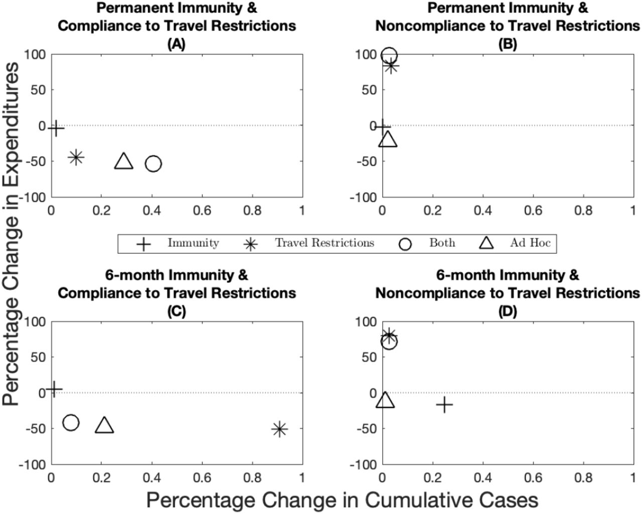
Percentage change in expenditures (y-axis) and percentage change in cumulative cases (x-axis) from the optimal allocation for different immunity–travel restrictions scenarios and for when vaccine capacity is 15%.
C.3.2 Heterogeneous Case-Fatality Ratio
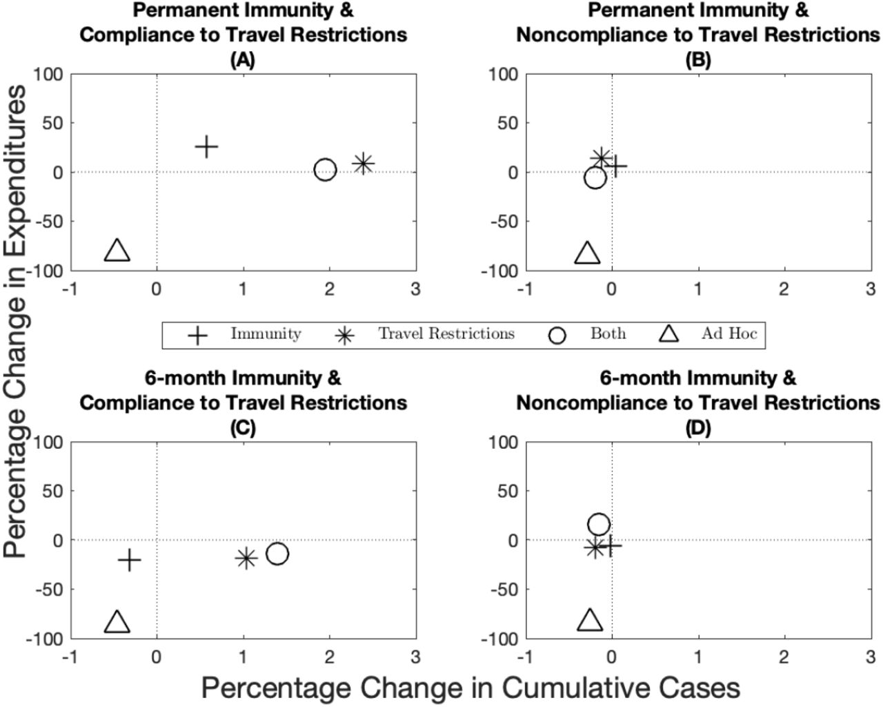
Percentage change in expenditures (y-axis) and percentage change in cumulative cases (x-axis) from the optimal allocation for different immunity–travel restrictions scenarios and for when vaccine capacity is 10%.

Percentage change in expenditures (y-axis) and percentage change in cumulative damages (x-axis) from the optimal allocation for different immunity–travel restrictions scenarios and for when vaccine capacity is 10%. Note that compared to Figure A15, the use of cumulative damages in this figure gives a more accurate depiction of the situation because cases across jurisdictions are not homogeneous when the case-fatality ratio is different.
C.3.3 Heterogeneous Contact Rate

Percentage change in expenditures (y-axis) and percentage change in cumulative cases (x-axis) from the optimal allocation for different immunity–travel restrictions scenarios and for when vaccine capacity is 10%.
C.4 Sensitivity Analyses
C.4.1 Workability Cost
As mentioned above, imposing the ad hoc rule ex ante implicitly means that the central planning agency is essentially assuming that the cost of deviating from the ad hoc allocation is infinite. In practice, the workability cost is hard to quantify, because it depends on logistical, political, and cultural factors. It does however seem reasonable to assume, as we did in the paper, that the cost is finite. We investigate the sensitivity of our results by solving for the optimal vaccine allocation over time with levels lower and higher than the base case parameter in the paper. We summarize these results by plotting the variance16 of the optimal deviation in each time period from the ad hoc vaccine allocation (in blue; Figure A18 panels A, B, C, and D), and the difference in cumulative cases between the optimal and ad hoc allocation (in red; Figure A18 panels A, B, C, and D) as we vary the scale of the workability cost. Mathematically, as the workability cost approaches zero, the optimal control problem becomes linear in the controls, which implies that there is no adjustment cost associated with changing the allocation. Often times this can lead to extreme solutions (allocation goes to one state for a time period and then the other state, and so on).
Given the behavior and nature of the problem, therefore, we expect that at lower values of the workability cost parameter we will find higher variance of the deviation. This, in turn results in a higher performance of the optimal allocation relative to the ad hoc in terms of reduction in cumulative cases. When we increase the workability cost parameter, the cost parameter will eventually be on the same magnitude as the VSL (Figure A18 black line represents the VSL). When we reach levels this high, the optimal allocation converges towards the ad hoc and any differences in cumulative cases disappear.
We also show how amount of funds allocated to the workability cost over time compare to expenditures on the total vaccine cost (Figure A18 panels E, F, G, and H). If this ratio exceeds one, the planner is spending on aggregate more to deviate from the ad hoc than on treatments. These panels show that at low levels of the workability cost parameter, the total workability costs are small relative to the total vaccine costs. As the workability cost parameter increases, however, the total workability costs become more and more important relative to the total vaccine cost. Eventually, these costs begin to dominate the planners objective and the deviation between the ad hoc and optimal goes to zero.
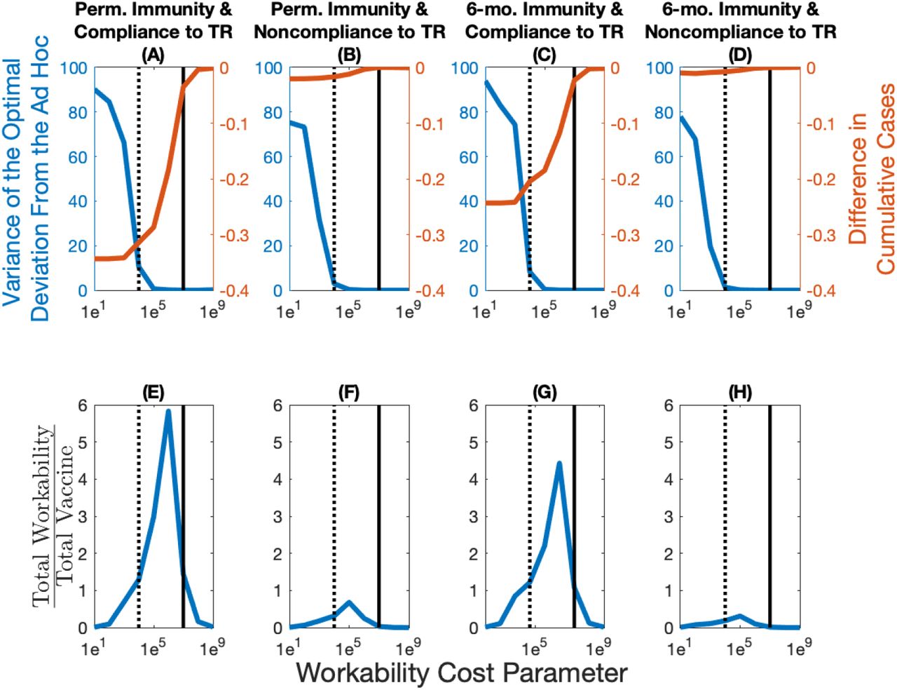
The variance of the optimal deviation in percentage (in blue; panels A, B, C, and D) represents an aggregate measure of the optimal deviation from the ad hoc allocation. The difference in cumulative cases between the optimal and ad hoc allocations (in red; panels A, B, C, and D) represents in percentage terms how well the optimal allocation outperforms the ad hoc allocation. The total workability cost over the total vaccine cost (panels E, F, G, and H) represents how many times more the total workability costs are relative to the total vaccine costs. The dotted vertical line represents the base case value of the workability cost parameter (1e4), while the full vertical line represents the value of statistical life (1e7).
C.4.2 Vaccine Effectiveness
The base case parameter for vaccine effectiveness we utilized in the paper is based on estimates of the influenza vaccine [15]; see Appendix A for more details. Recent evidence from the COVID-19 vaccines suggest that effectiveness could be considerably higher. As a result, we investigate how a more effective vaccine would affect the nature of our results. We find that the more effective a vaccine is, the more a central planner would want to deviate from the ad hoc allocation (in blue; Figure A19 panels A, B, C, and D). As a result of this greater deviation, we see a larger difference in terms of the reduction in cumulative cases (in red; Figure A19 panels A, B, C, and D). Because a higher effectiveness results in a greater deviation, then, everything else equal, the total workability costs are increased relative to the total vaccine costs (Figure A19 panels E, F, G, and H). The differences are more stark in a world where there is compliance to travel restrictions, as noncompliance blurs the spatial heterogeneity across the jurisdictions leading in general to allocations similar to the ad hoc.

The variance of the optimal deviation in percentage (in blue; panels A, B, C, and D) represents an aggregate measure of the optimal deviation from the ad hoc allocation. The difference in cumulative cases between the optimal and ad hoc allocations (in red; panels A, B, C, and D) represents in percentage terms how well the optimal allocation outperforms the ad hoc allocation. The total workability cost over the total vaccine cost (panels E, F, G, and H) represents how many times more the total workability costs are relative to the total vaccine costs. The dotted vertical line in the plots represents the base case value of the vaccine effectiveness (0.65).
Footnotes
† We thank for useful comments participants of the NatuRE Policy Lab at UC Davis (naturepolicy.ucdavis.edu), as well as participants of the internal seminars of the Department of Economics at Université du Québec à Montréal (UQAM), and those of the Montreal Environment and Resource Economics Workshop.
‡ For the code used in this paper, see: https://github.com/fmcastonguay/SpatialAllocationCOVID19
Removed the section on antivirals and focussed the discussion more around vaccines and heterogeneous demographic characteristics.
↵1 See “What value of statistical life does EPA use?” from the U.S. Environmental Protection Agency [9].
↵2 According to the World Health Organization: “A disability weight is a weight factor that reflects the severity of the disease on a scale from 0 (perfect health) to 1 (equivalent to death).” See: https://www.who.int/healthinfo/global_burden_disease/daly_disability_weight/en/.
↵3 For more details on how COVID-19’s disability resembles lower respiratory tract infections, see [10].
↵4 For COVID-19 vaccine prices, see: https://www.npr.org/sections/health-shots/2020/08/06/899869278/prices-for-covid-19-vaccines-are-starting-to-come-into-focus. For a comparison with influenza vaccine prices, see https://www.cdc.gov/vaccines/programs/vfc/awardees/vaccine-management/price-list/index.html.
↵5 Inspired by the paper of Ryan et al. [11] where the authors show the implications of policy adjustment costs for fisheries management
6 Calibrated using a R0 estimate from Li et al. [4] and estimates of effects of nonpharmaceutical interventions from Tian et al. [5]; this yields a R0 of approximately 1.4 when there is compliance to travel restrictions and to match a R0 of approximately 2.1 when there is no compliance to travel restrictions; these two values representing respectively a “medium” and “low” effect of the nonpharmaceutical intervention.
7 Using estimates from Davies et al. [6]; this represents a 3-day latency period and a 5-day recovery period.
8 Representing a 6-month immunity period in the scenarios where we assume immunity is not permanent; based on [13].
9 Calibrated by using a case-fatility rate of 1.78%. Adjusted for mis- and under-reporting; see [7].
10 Representing the disability associated with severe lower respiratory tract infections because, to our knowledge, there are no official disability estimates associated with COVID-19; see [10].
11 Following Buckner et al. [14], we base this parameter value on the efficiency of the influenza vaccine [15]. Note that the Department of Health and Human Services, Food and Drug Administration (FDA), and Center for Biologics Evaluation and Research (CBER) [16] requires that a future COVID-19 vaccine must have an effectiveness of at least 50%.
12 Based on results from John et al. [12] that suggest a yearly discount rate between 0.3% and 1.5% for health related expenditures; we chose a 1.5% annual discount rate in the main set of results. This gives a monthly discount rate of r = 0.0013.
13 Assuming an individual requires two doses; based on current agreements between the U.S. federal government and biotech companies; see https://www.npr.org/sections/health-shots/2020/08/06/899869278/prices-for-covid-19-vaccines-are-starting-to-come-into-focus. For a list of current vaccine prices, and particularly the price of the influenza vaccine, see https://www.cdc.gov/vaccines/programs/vfc/awardees/vaccine-management/price-list/index.html.
14 Value based on a certain proportion of the value of statistical life, c; in the base case we assume it is 2 orders of magnitude smaller.
15 Represents a value of statistical life of 10M U.S. dollars. Based on the value of a statistical life that the U.S. Environmental Protection Agency [9] uses: approximately $7.4 million ($2006) which is equivalent to approximately $9.54 million ($2020).
↵16 The variance is calculated as Var
 . Note that the variance of the optimal deviation from the ad hoc is identical in absolute and relative terms across jurisdictions.
References
- [1].↵
- [2].↵
- [3].↵
- [4].↵
- [5].↵
- [6].↵
- [7].↵
- [8].↵
- [9].↵
- [10].↵
- [11].↵
- [12].↵
- [13].↵
- [14].↵
- [15].↵
- [16].↵
- [17].↵
- [18].↵
- [19].↵
- [20].↵
- [21].↵
- [22].↵
- [23].↵
- [24].↵
- [25].↵
- [26].↵
- [27].↵
- [28].↵
- [29].↵
- [30].↵
- [31].↵
- [32].↵
- [33].↵
- [34].↵
- [35].↵
- [36].↵
- [37].↵
- [38].↵
- [39].↵
- [40].↵
- [41].↵
- [42].↵
- [43].↵
- [44].↵
- [45].↵
- [46].↵
- [47].↵
- [48].↵
- [49].↵
- [50].↵
- [51].↵
- [52].↵
- [53].↵
- [54].↵
- [55].↵
- [56].↵


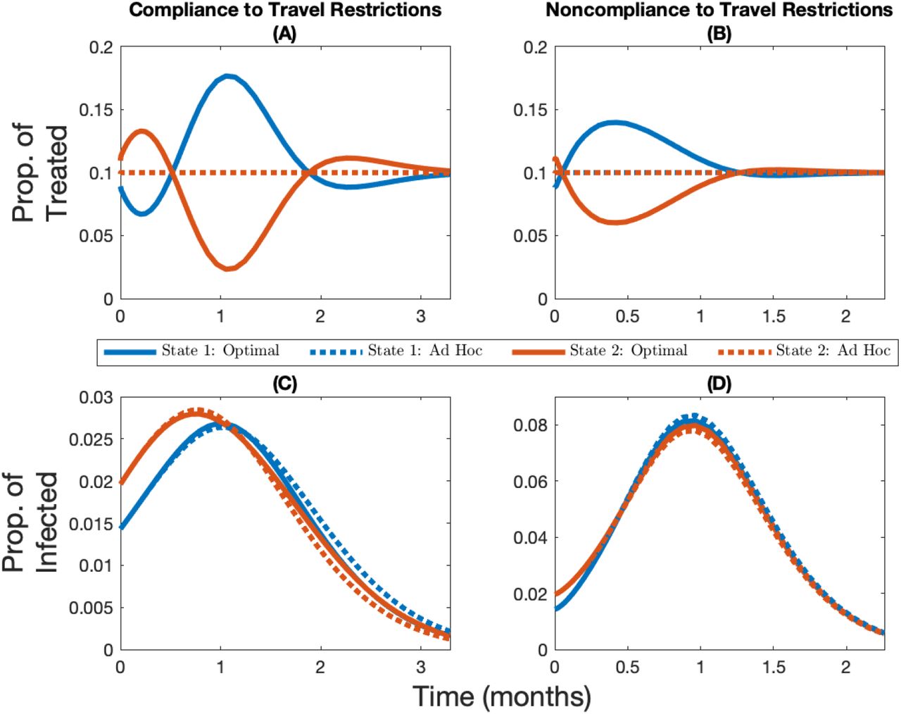
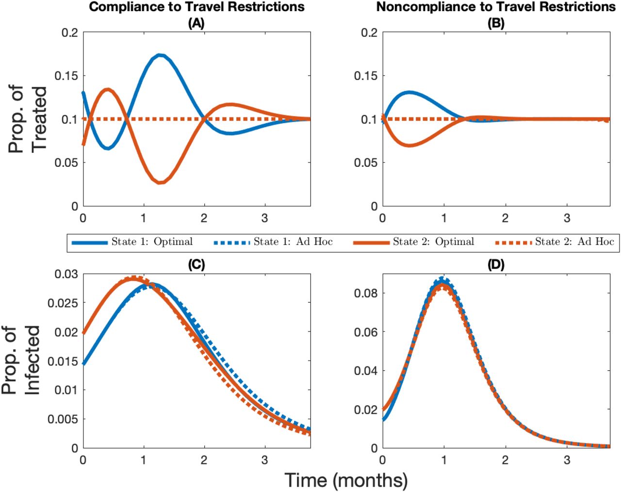
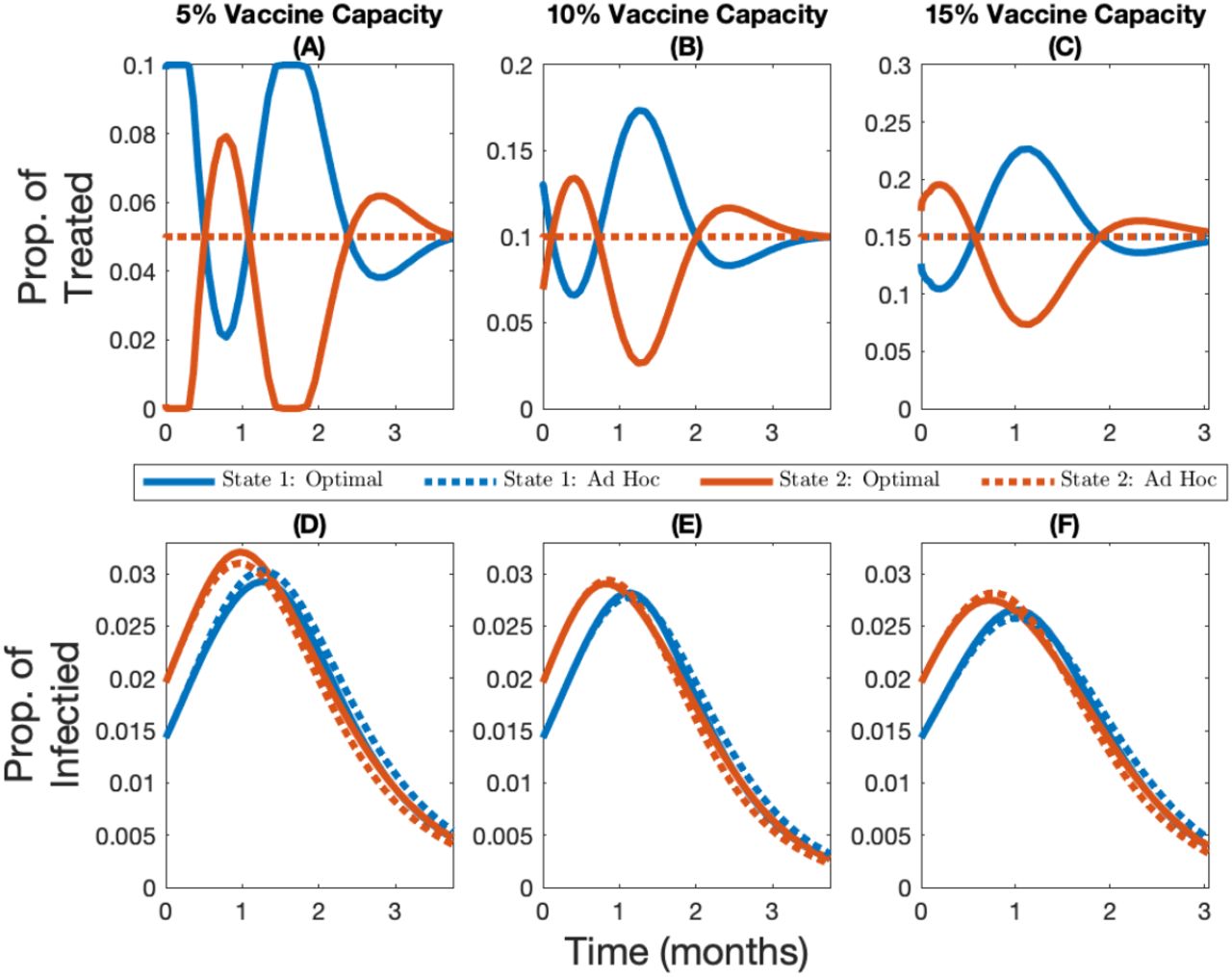
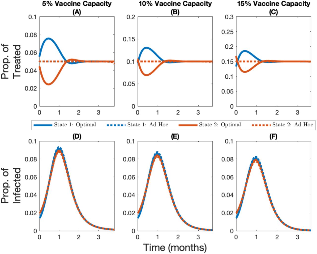
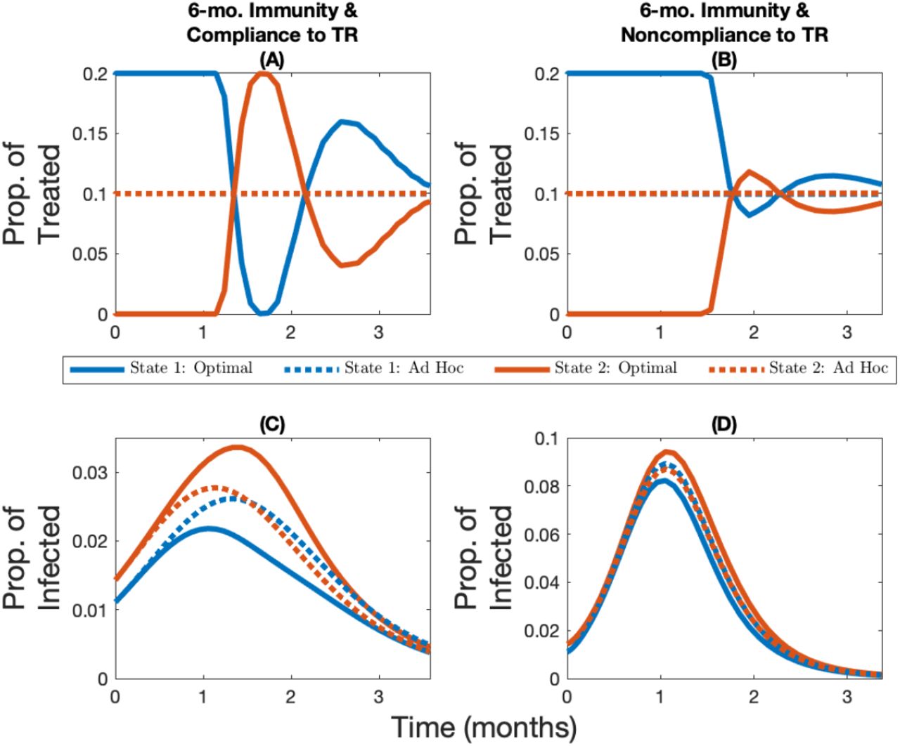
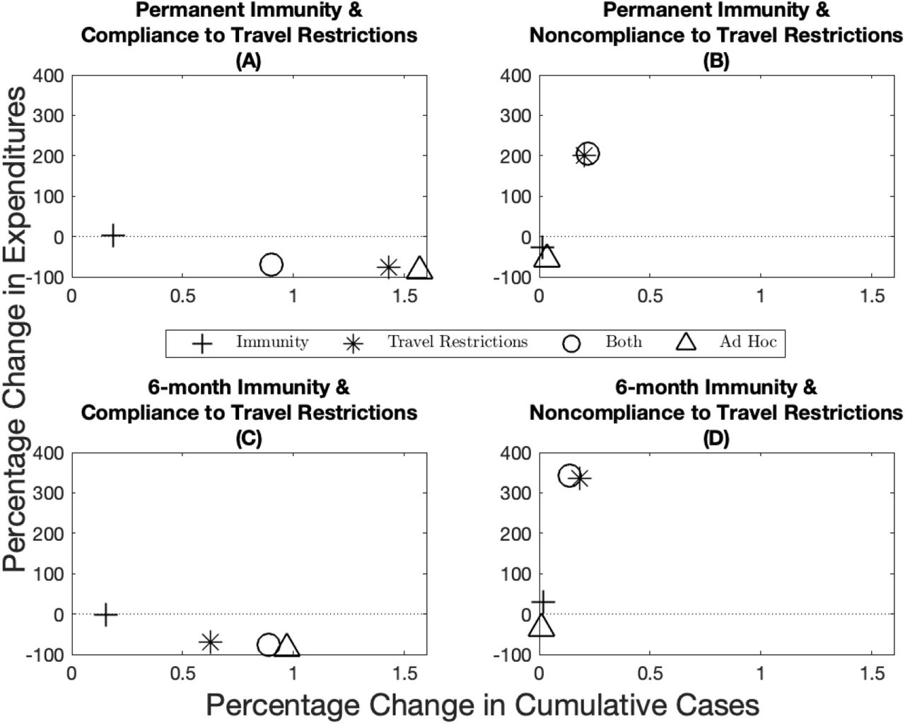