
Abstract
Background SARS-CoV-2 infections are characterized by viral proliferation and clearance phases and can be followed by low-level viral RNA shedding. The dynamics of viral RNA concentration, particularly in the early stages of infection, can inform clinical measures and interventions such as test-based screening.
Methods We used prospective longitudinal RT-qPCR testing to measure the viral RNA trajectories for 68 individuals during the resumption of the 2019-20 National Basketball Association season. For 46 individuals with acute infections, we inferred the peak viral concentration and the duration of the viral proliferation and clearance phases.
Findings On average, viral RNA concentrations peaked 2.7 days (95% credible interval [1.2, 3.8]) after first detection at a cycle threshold value of 22.4 [20.6, 24.1]. The viral clearance phase lasted longer for symptomatic individuals (10.5 days [6.5, 14.0]) than for asymptomatic individuals (6.7 days [3.2, 9.2]). A second test within 2 days after an initial positive PCR substantially improves certainty about a patient’s infection phase. The effective sensitivity of a test intended to identify infectious individuals declines substantially with test turnaround time.
Interpretation SARS-CoV-2 viral concentrations peak rapidly regardless of symptoms. Sequential tests can help reveal a patient’s progress through infection stages. Frequent rapid-turnaround testing is needed to effectively screen individuals before they become infectious.
Funding NWO Rubicon 019.181EN.004 (CBFV); clinical research agreement with the NBA and NBPA (NDG); Huffman Family Donor Advised Fund (NDG); Fast Grant funding from the Emergent Ventures at the Mercatus Center; George Mason University (NDG); the Morris-Singer Fund for the Center for Communicable Disease Dynamics at the Harvard T.H. Chan School of Public Health (YHG).
Evidence before this study SARS-CoV-2 viral dynamics affect clinical and public health measures, informing patient care, testing algorithms, contact tracing protocols, and clinical trial design. We searched Web of Science using the search terms “ALL = ((SARS-CoV-2 OR COVID-19) AND (viral OR RNA) AND (load OR concentration OR shedding) AND (dynamic* OR kinetic* OR trajector*))” which returned 83 references. Of these, 22 were not pertinent to within-host SARS-CoV-2 viral dynamics. The remaining 61 studies tracked SARS-CoV-2 viral trajectories in a variety of geographic locations and patient populations. Together, these studies report that viral titers normally peak at or before the onset of symptoms and that a long tail of intermittent positive tests can follow a period of acute infection. Plasma but not nasopharyngeal viral concentration is associated with increased disease severity. Most studies tracked hospitalized patients after the onset of symptoms. Two of the studies tracked pre-symptomatic and/or asymptomatic patients, but these were too sparsely sampled to clearly discern viral dynamics during the earliest stage of infection.
Added value of this study We implemented prospective longitudinal real time quantitative reverse transcriptase polymerase chain reaction (RT-qPCR) testing for SARS-CoV-2 in a cohort of individuals during the resumption of the 2019-20 National Basketball Association season. This allowed us to explicitly measure viral titers during the full course of 46 acute infections. Consistent with other studies, we find that peak viral concentrations do not differ substantially between symptomatic and asymptomatic individuals but that symptomatic individuals take longer to clear the virus than asymptomatic individuals. For both symptomatic and asymptomatic individuals, viral titers normally peak within 3 days of the first positive test. This study is the first to describe the time course of viral concentrations during the earliest stage of infection when individuals are most likely to be infectious.
Implications of all the available evidence Symptomatic and asymptomatic individuals follow similar SARS-CoV-2 viral trajectories. Due to the rapid progression from first possible detection to peak viral concentration, frequent rapid-turnaround testing is needed to screen individuals prior to them becoming infectious.
Introduction
As mortality from the COVID-19 pandemic surpasses one million, SARS-CoV-2 continues to cause hundreds of thousands of daily new infections1. A critical strategy to curb the spread of the virus without imposing widespread lockdowns is to rapidly identify and isolate infectious individuals. Because symptoms are an unreliable indicator of infectiousness and infections are frequently asymptomatic2, testing is key to determining whether a person is infected and may be contagious.
Real time quantitative reverse transcriptase polymerase chain reaction (RT-qPCR) tests are the gold standard for detecting SARS-CoV-2 infection. Normally, these tests yield a binary positive/negative diagnosis based on detection of viral RNA. However, they can also quantify the viral titer via the cycle threshold (Ct). The Ct is the number of thermal cycles needed to amplify sampled viral RNA to a detectable level: the higher the sampled viral RNA concentration, the lower the Ct. This inverse correlation between Ct and viral concentration makes RT-qPCR tests far more valuable than a binary diagnostic, as they can be used to reveal a person’s progress through key stages of infection3, with the potential to assist clinical and public health decision-making. However, the dynamics of the Ct during the earliest stages of infection, when contagiousness is rapidly increasing, have been unclear, because diagnostic testing is usually performed after the onset of symptoms, when viral RNA concentration has peaked and already begun to decline, and performed only once4,5. Without a clear picture of the course of SARS-CoV-2 viral concentrations across the full duration of acute infection, it has been impossible to specify key elements of testing algorithms such as the frequency rapid at-home testing6 that will be needed to reliably screen infectious individuals before they transmit infection. Here, we fill this gap by analyzing the prospective longitudinal SARS-CoV-2 RT-qPCR testing performed for players, staff, and vendors during the resumption of the 2019-20 National Basketball Association (NBA) season.
Methods
Data collection
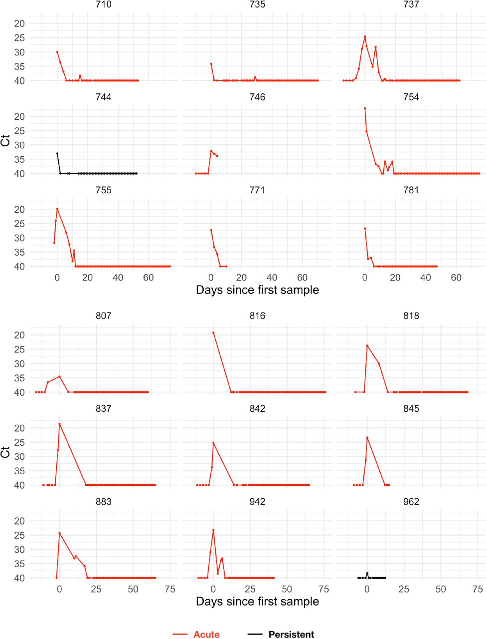
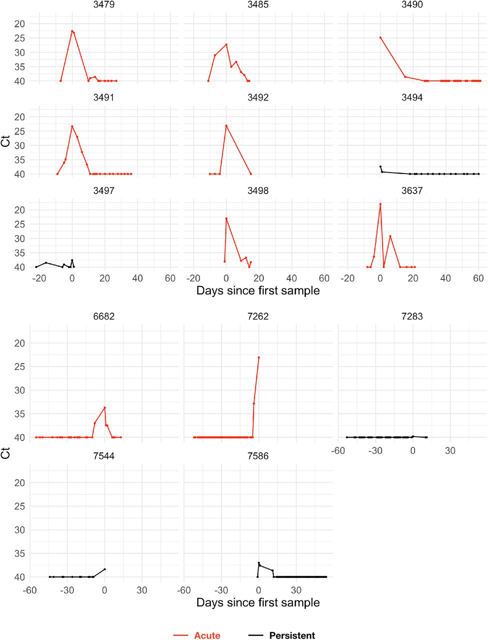
The study period began in teams’ local cities from June 23rd through July 9th, 2020, and testing continued for all teams as they transitioned to Orlando, Florida through September 7th, 2020. A total of 68 individuals (90% male) were tested at least five times during the study period and recorded at least one positive test with Ct value <40. Many individuals were being tested daily as part of Orlando campus monitoring. Due to a lack of new infections among players and team staff after clearing quarantine in Orlando, all players and team staff included in the results pre-date the Orlando phase of the restart. A diagnosis of “acute” or “persistent” infection was abstracted from physician records. “Acute” denoted a likely new infection. “Persistent” indicated the presence of virus in a clinically recovered individual, likely due to infection that developed prior to the onset of the study. There were 46 acute infections; the remaining 22 individuals were assumed to be persistently shedding SARS-CoV-2 RNA due to a known infection that occurred prior to the study period. This persistent RNA shedding can last for weeks after an acute infection and likely represented non-infectious viral RNA7. Of the individuals included in the study, 27 of the 46 with acute infections and 40 of the 68 overall were from staff and vendors. The Ct values for all tests for the 68 individuals included in the analysis with their designations of acute or persistent infection are depicted in Supplemental Figures 1–4. A schematic diagram of the data collection and analysis pipeline is given in Figure 1.
Statistical analysis
We used a Bayesian statistical model to infer the peak Ct value and the durations of the proliferation and clearance stages for the 46 acute infections with at least on Ct value below 35 (Figure 1; Supplemental Methods). We assumed that the viral concentration trajectories consisted of a proliferation phase, with exponential growth in viral RNA concentration, followed by a clearance phase characterized by exponential decay in viral RNA concentration8. Since Ct values are roughly proportional to the negative logarithm of viral concentration3, this corresponds to a linear decrease in Ct followed by a linear increase. We therefore constructed a piecewise-linear regression model to estimate the peak Ct value, the time from infection onset to peak (i.e., the duration of the proliferation stage), and the time from peak to infection resolution (i.e., the duration of the clearance stage). We estimated the parameters of the regression model by fitting to the available data using a Hamiltonian Monte Carlo algorithm9 yielding simulated draws from the Bayesian posterior distribution for each parameter. Full details on the fitting procedure are given in the Supplemental Methods. Code is available at https://github.com/gradlab/CtTrajectories.
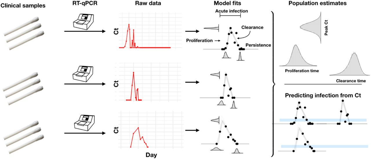
Combined anterior nares and oropharyngeal swabs were tested using a RT-qPCR assay to generate longitudinal Ct values (‘Raw data’, red points) for each person. Using a statistical model, we estimated Ct trajectories consistent with the data, represented by the thin lines under the ‘Model fits’ heading. These produced posterior probability distributions for the peak Ct value, the duration of the proliferation phase (infection onset to peak Ct), and the duration of the clearance phase (peak Ct to resolution of acute infection) for each person. We estimated population means for these quantities. The model fits also allowed us to determine how frequently a given Ct value or pair of Ct values within a five-unit window (blue bars, bottom-right pane) was associated with the proliferation phase, the clearance phase, or a persistent infection.
Inferring stage of infection
Next, we determined whether individual or paired Ct values can reveal whether an individual is in the proliferation, clearance, or persistent stage of infection. To do so, we extracted all observed Ct values within a 5-unit window (e.g., between 30 and 35 Ct) and measured how frequently these values sat within the proliferation stage, the clearance stage, or the persistent stage. We measured these frequencies across 10,000 posterior parameter draws to account for that fact that Ct values near stage transitions (e.g., near the end of the clearance stage) could be assigned to different infection stages depending on the parameter values (see Figure 1, bottom-right). We did this for 23 windows with midpoint spanning from Ct = 37.5 to Ct = 15.5 in increments of 1 Ct.
To calculate the probability that a Ct value falling within the 5-unit window corresponded to an acute infection (i.e., either the proliferation or the clearance stage), we summed the proliferation and clearance frequencies for all samples within that window and divided by the total number of samples in the window. We similarly calculated the probability that a Ct falling within the 5-unit window corresponded to just the proliferation phase.
To assess the information gained by conducting a second test within two days of an initial positive, we restricted our attention to all samples within the 5-unit window that had a subsequent sample taken within two days. We repeated the above calculations, stratifying by whether the second test had a higher or lower Ct than the first.
Measuring the effective sensitivity of screening tests
The sensitivity of a test is defined as the probability that the test correctly identifies an individual who is positive for some criterion of interest. For clinical diagnostic SARS-CoV-2 tests, the criterion of interest is current infection with SARS-CoV-2. However, a common goal is to predict infectiousness at some point in the future, as in the context of test-based screening prior to a social gathering. The ‘effective sensitivity’ of a test in this context (i.e., its ability to predict future infectiousness) may differ substantially from its clinical sensitivity (i.e., its ability to detect current infection). A test’s effective sensitivity depends on its inherent characteristics, such as its limit of detection and sampling error rate, as well as the viral dynamics of infected individuals.
To illustrate this, we estimated the effective sensitivity of (a) a test with limit of detection of 40 Ct and a 1% sampling error probability (akin to RT-qPCR), and (b) a test with limit of detection of 35 Ct a 5% sampling error probability (akin to some rapid antigen tests). We measured the frequency with which these tests would successfully screen an individual who would become infectious (assumed to correspond to Ct ≤ 30) 10 at the time of a gathering when the test was administered between 0 and 3 days prior to the gathering. We measured this effective sensitivity with respect to 2,500 simulated viral concentration trajectories sampled from the posterior distributions from the best-fit model, restricting to trajectories with peak Ct below 30 (any samples with peak Ct > 30 would, by these criteria, never be infectious and so would not factor into the sensitivity calculation). Full details are given in the Supplemental Methods.
We also estimated the number of individuals who would be expected to arrive at a 1,000-person gathering while infectious assuming a 2% prevalence of infectiousness in the population under each testing strategy. To do so, we simulated 1,000 events for which the number of infectious individuals at the event was simulated using a Binomial distribution with 1,000 draws and ‘success’ probability of 0.02. Then, we sampled the number of these infectious individuals who would be screened using a second Binomial draw with ‘success’ probability dictated by the previously calculated effective sensitivity. Further details are given in the Supplemental Methods. To facilitate the exploration of different scenarios, we have generated an online tool (https://stephenkissler.shinyapps.io/shiny/) where users can input test and population characteristics and calculate the effective sensitivity and expected number of infectious individuals at a gathering.
Results
Of the 46 individuals with acute infections, 13 reported symptoms at the time of diagnosis; the timing of the onset of symptoms was not recorded. The mean peak Ct value for symptomatic individuals was 22.2 (95% credible interval [19.1, 25.1]), the mean duration of the proliferation phase was 2.9 days [0.7, 4.7], and the mean duration of clearance was 10.5 days [6.5, 14.0] (Figure 2). This compares with 22.4 Ct [20.2, 24.5], 3.0 days [1.3, 4.3], and 6.7 days [3.2, 9.2], respectively, for individuals who did not report symptoms at the time of diagnosis (Figure 2). This yielded a slightly longer overall duration of acute infection for individuals who reported symptoms (13.4 days [9.3, 17.1]) vs. those who did not (9.7 days [6.0, 12.5]). For all individuals regardless of symptoms, the mean peak Ct value, proliferation duration, clearance duration, and duration of acute shedding were 22.4 Ct [20.6, 24.1], 2.7 days [1.2, 3.8], 7.4 days [3.9, 9.6], and 10.1 days [6.5, 12.6] (Supplemental Figure 5). There was a substantial amount of individual-level variation in the peak Ct value and the proliferation and clearance stage durations (Supplemental Figures 6–11).
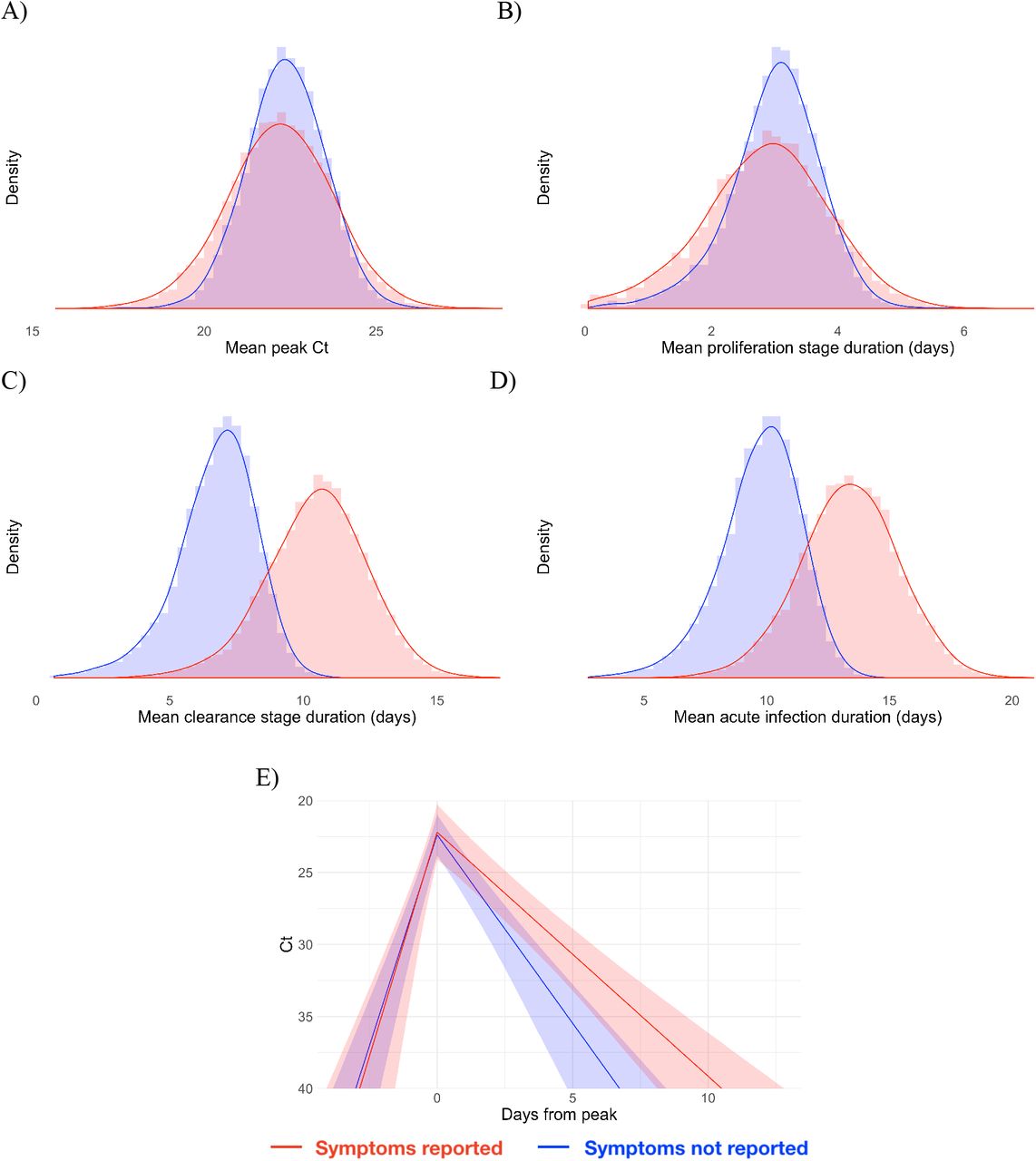
Histograms (colored bars) of 10,000 simulated draws from the posterior distributions for mean peak Ct value (A), mean duration of the proliferation stage (infection detection to peak Ct, B), mean duration of the clearance stage (peak Ct to resolution of acute RNA shedding, C), and total duration of acute shedding (D) across the 46 individuals with an acute infection. The histograms are separated according to whether the person reported symptoms (red, 13 individuals) or did not report symptoms (blue, 33 individuals). The red and blue curves are kernel density estimators for the histograms to assist with visualizing the shapes of the histograms. The mean Ct trajectory corresponding to the mean values for peak Ct, proliferation duration, and clearance duration for symptomatic vs. asymptomatic individuals is depicted in (E) (solid lines), where shading depicts the 90% credible intervals.
Using the full dataset of 68 individuals, we estimated the frequency with which a given Ct value was associated with an acute infection (i.e., the proliferation or clearance phase, but not the persistence phase), and if so, the probability that it was associated with the proliferation stage alone. The probability of an acute infection increased rapidly with decreasing Ct (increasing viral load), with Ct < 30 virtually guaranteeing an acute infection in this dataset (Figure 3A). However, a single Ct value provided little information about whether an acute infection was in the proliferation or the clearance stage (Figure 3B).
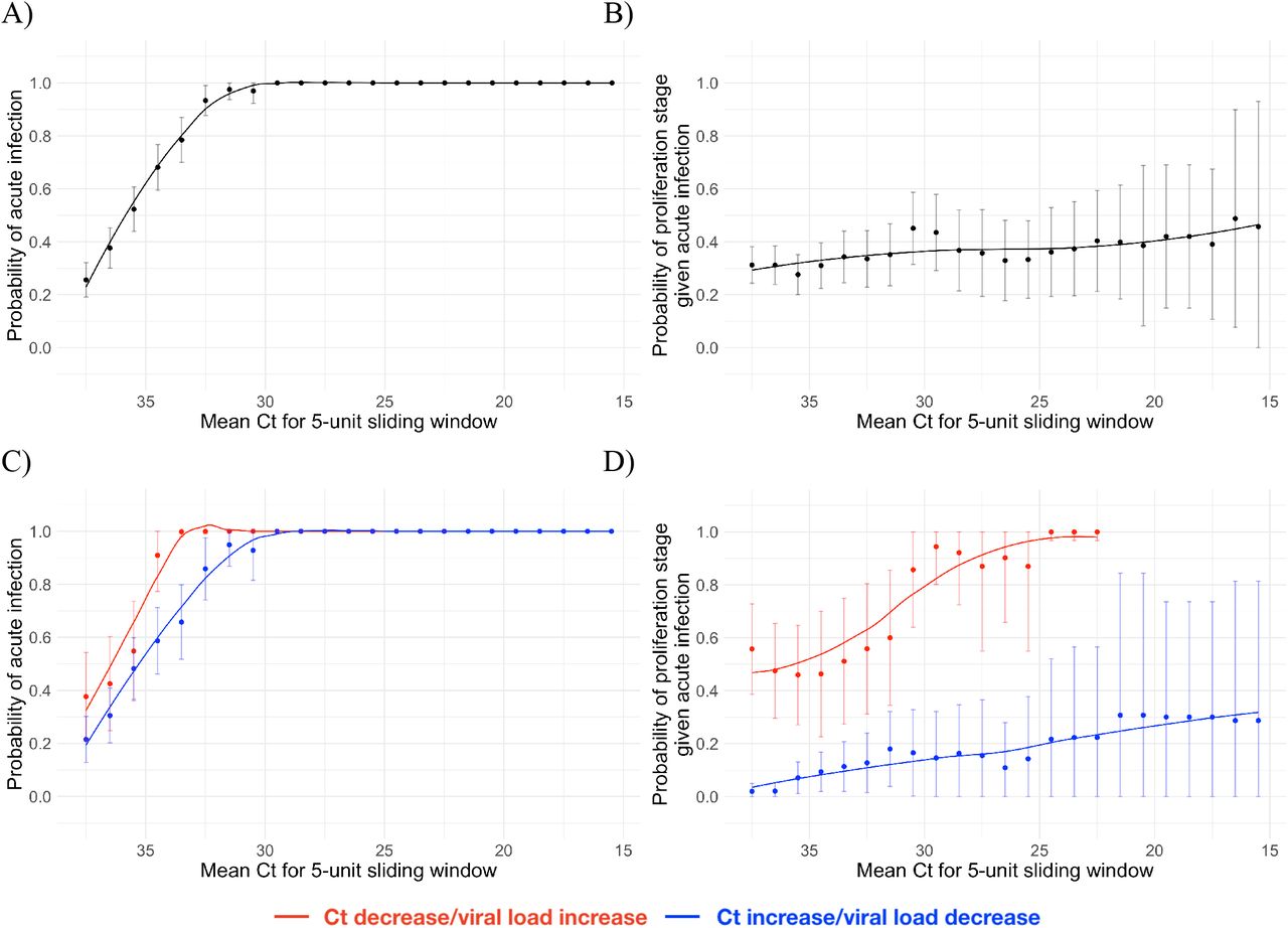
Probability that a given Ct value lying within a 5-unit window (horizontal axis) corresponds to an acute infection (A, C) or to the proliferation phase of infection assuming an acute infection (B, D). Sub-figures A and B depict the predictive probabilities for a single Ct value, while sub-figures C and D depict the predictive probabilities for a positive test paired with a subsequent test with either lower (red) or higher (blue) Ct. The curves are LOESS smoothing curves to better visualize the trends. Error bars represent the 90% Wald confidence interval.
We assessed whether a second test within two days of the first could improve these predictions. A positive test followed by a second test with lower Ct (higher viral RNA concentration) was slightly more likely to be associated with an active infection than a positive test alone (Figure 3C). Similarly, a positive test followed by a second test with lower Ct (higher viral RNA concentration) was much more likely to be associated with the proliferation phase than with the clearance phase (Figure 3D).
We next estimated how the effective sensitivity of a pre-event screening test declines with increasing time to the event. For a test with limit of detection of 40 Ct and a 1% chance of sampling error, the effective sensitivity declines from 99% when the test coincides with the start of the event to 76% when the test is administered two days prior to the event (Figure 4A), assuming a threshold of infectiousness at 30 Ct10. This two-day-ahead sensitivity is slightly lower than the effective sensitivity of a test with a limit of detection at 35 Ct and a 5% sampling error administered one day before the event (82%), demonstrating that limitations in testing technology can be compensated for by reducing turnaround time. Using these effective sensitivities, we estimated the number of infectious individuals expected to arrive at an event with 1,000 people when 2% of the population is infectious. Just as the effective sensitivity declines with time to the event, the predicted number of infectious individuals rises (Figure 4B).
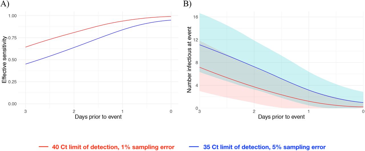
Effective sensitivity for a test with limit of detection of 40 Ct and 1% sampling error probability (red) and 35 Ct and 5% sampling error probability (blue) (A). Number of infectious individuals expected to attend an event of size 1000 assuming a population prevalence of 2% infectious individuals for a test with limit of detection of 40 Ct and 1% sampling error probability (red) and 35 Ct and 5% sampling error probability (blue). Shaded bands represent 90% prediction intervals generated from the quantiles of 1,000 simulated events and capture uncertainty both in the number of infectious individuals who would arrive at the event in the absence of testing and in the probability that the test successfully identifies infectious individuals.
Discussion
This report provides first comprehensive data on the early-infection RT-qPCR Ct dynamics associated with SARS-CoV-2 infection. Viral titers increase quickly, normally within 3 days of the first possible RT-qPCR detection, regardless of symptoms. Our findings highlight that repeated PCR tests can be used to infer the stage of a patient’s infection. While a single test can inform on whether a patient is in the acute or persistent viral RNA shedding stages, a subsequent test can help identify whether viral RNA concentrations are increasing or decreasing, thus informing clinical care. We also show that the effective sensitivity of pre-event screening tests declines rapidly with test turnaround time due to the rapid progression from detectability to peak viral titers. Due to the transmission risk posed by large gatherings11, the trade-off between test speed and sensitivity must be weighed carefully. These data offer the first direct measurements capable of informing such decisions.
Our findings on the duration of SARS-CoV-2 viral RNA shedding expand on and agree with previous studies12,13 and with observations that peak Ct does not differ substantially between symptomatic and asymptomatic individuals4. While previous studies have largely relied on serial sampling of admitted hospital patients, our study used prospective sampling of ambulatory infected individuals to characterize complete viral dynamics for the presymptomatic stage and for individuals who did not report symptoms. This allowed us to assess differences between the viral RNA proliferation and clearance stages for individuals with and without reported symptoms. The similarity in the early-infection viral RNA dynamics for both symptomatic and asymptomatic individuals underscores the need for SARS-CoV-2 screening regardless of symptoms. The rapid progression from a negative test to a peak Ct value 2-4 days later provides empirical support for screening and surveillance strategies that employ frequent rapid testing to identify potentially infectious individuals14,15. Taken together, the dynamics of viral RNA shedding substantiate the need for frequent population-level SARS-CoV-2 screening and a greater availability of diagnostic tests.
Our findings are limited for several reasons. The cohort does not constitute a representative sample from the population, as it was a predominantly male, healthy, young population inclusive of professional athletes. Some of the trajectories were sparsely sampled, limiting the precision of our posterior estimates. Symptom reporting was imperfect, particularly after initial evaluation as follow-up during course of disease was not systematic for all individuals. As with all predictive tests, the probabilities that link Ct values with infection stages (Figure 3) pertain to the population from which they were calibrated and do not necessarily generalize to other populations for which the prevalence of infection and testing protocols may differ. Still, we anticipate that the central patterns will hold across populations: first, that low Cts (<30) strongly predict acute infection, and second, that a follow-up test collected within two days of an initial positive test can substantially help to discern whether a person is closer to the beginning or the end of their infection. Our study did not test for the presence of infectious virus, though previous studies have documented a close inverse correlation between Ct values and culturable virus10. Our assessment of pre-event testing assumed that individuals become infectious immediately upon passing a threshold and that this threshold is the same for the proliferation and for the clearance phase. In reality, the threshold for infectiousness is unlikely to be at a fixed viral concentration for all individuals and may be at a higher Ct/lower viral concentration during the proliferation stage than during the clearance stage. Further studies that measure culturable virus during the various stages of infection and that infer infectiousness based on contact tracing combined with prospective longitudinal testing will help to clarify the relationship between viral concentration and infectiousness.
To manage the spread of SARS-CoV-2, we must develop novel technologies and find new ways to extract more value from the tools that are already available. Our results suggest that integrating the quantitative viral RNA trajectory into algorithms for clinical management could offer benefits. The ability to chart a patient’s progress through their infection underpins our ability to provide appropriate clinical care and to institute effective measures to reduce the risk of onward transmission. Marginally more sophisticated diagnostic and screening algorithms may greatly enhance our ability to manage the spread of SARS-CoV-2 using tests that are already available.
Data Availability
Code and data are available at https://github.com/gradlab/CtTrajectories
Supplemental Methods
Ethics
Residual de-identified viral transport media from anterior nares and oropharyngeal swabs collected NBA players, staff, and vendors were obtained from Quest Diagnostics or BioReference Laboratories. In accordance with the guidelines of the Yale Human Investigations Committee, this work with de-identified samples was approved for research not involving human subjects by the Yale Internal Review Board (HIC protocol # 2000028599). This project was designated exempt by the Harvard IRB (IRB20-1407).
Additional testing protocol details
Clinical samples were obtained by combined swabs of the anterior nares and oropharynx administered by a trained provider. The samples were initially tested by either Quest Diagnostics (while teams were in local markets using the Quest SARS-CoV-2 RT-qPCR16) or BioReference Laboratories (while teams were in Orlando using the cobas SARS-CoV-2 test17). Viral transport media from positive samples were sent to Yale University for subsequent RT-qPCR testing using a multiplexed version of the assay from the US Centers for Disease Control and Prevention 18 to normalize Ct values across testing platforms. A total of 234 samples from BioReference and 128 from Quest were tested at Yale; 49 positive samples had Ct values assigned on first testing but did not undergo repeat testing at the Yale laboratory. To account for the different calibration of the testing instruments, we used a linear conversion (Supplemental Figures 12-14, Methods: Converting Ct values) to adjust these samples to the Yale laboratory scale. Subsequent analysis is based on the N1 Ct value from the Yale multiplex assay and on the adjusted Roche cobas target 1 assay.
Residual viral transport media (VTM) from Quest Diagnostics or BioReference Laboratories were shipped overnight to Yale on dry ice. VTM was thawed on ice and 300 µL was used for RNA extraction using the MagMAX Viral/Pathogen Nucleic Acid Isolation Kit and the KingFisher Flex robot (Thermo Fisher Scientific, Waltham, MA19). Total nucleic acid was eluted into 75ul of elution buffer and SARS-CoV-2 RNA was quantified from 5 µL of extracted total RNA using a multiplexed version of the CDC RT-qPCR assay that contains the 2019-nCoV_N1 (N1), 2019-nCoV-N2 (N2), and human RNase P (RP) primer-probe sets18. The RT-qPCR was performed using the Luna Universal Probe One-Step RT-qPCR Kit (New England Biolabs, Ipswich, MA, US) and the following thermocycler conditions: (1) reverse transcription for 10 minutes at 55°C, (2) initial denaturation for 1 min at 95°C, and PCR for 45 cycles of 10 seconds at 95°C and 30 seconds at 55°C on the CFX96 qPCR machine (Bio-Rad, Hercules, CA, US).
Converting Ct values
Most (n = 226) of the 312 positive samples in the raw dataset underwent RT-qPCR at the Yale laboratory. We used the Yale Ct value whenever it was available. Still, 86 samples underwent initial diagnostic testing at BioReference Laboratories but not confirmatory testing at the Yale laboratory. Both platforms rely on a multiplex RT-qPCR strategy. The two testing platforms yield slightly different Ct values, as evidenced by the 94 samples the underwent RT-qPCR at both facilities (Supplemental Figure 12). For comparison between platforms, target 1 from the Roche cobas assay, which is specific to SARS-CoV-2, and the N1 target from the Yale multiplex assay were used. For the 86 samples that were not processed at the Yale laboratory, we adjusted the Ct values using the best-fit (minimum sum of squares) linear regression between the initial Ct value and the Yale Ct value for the samples that were processed in both facilities. To do so, we estimated the coefficients β0 and β1 in the following regression equation:
Here, yi denotes the ith Ct value from Yale, xi denotes the ith Ct value from the initial test, and εi is an error term with mean 0 and constant variance across all samples. The resulting fit (Supplemental Figure 12) was strong (R2 = 0.86) with homoscedastic residuals (Supplemental Figure 13) that are approximately normally distributed, as evidenced by a Q-Q plot (Supplemental Figure 14).
Data parsing
The raw dataset included 3,207 test results for 102 individuals. We excluded 21 individuals who had 5 or fewer tests, since the data for these individuals were too sparse to reliably infer a Ct trajectory. We also excluded 13 individuals who did not record any Ct values that surpassed the RT-qPCR limit of detection (40). We removed 146 entries for which the test result was recorded as ‘positive’ but there was no associated Ct value; these tests were initially conducted on an instrument that provided only a binary diagnosis and the samples were not available for confirmatory testing. This left 2,411 total tests for 68 individuals for the main analysis. The median number of tests administered to each of the 68 individuals was 41 (IQR [14, 51]; Range [5, 70]). The median number of Ct values with viral concentration above the limit of detection recorded for each person was 3 (IQR [2, 4]; Range [1, 9]). We trivially shifted the date indices so that date 0 corresponded to the time of the minimum Ct. We set the Ct value for negative tests equal to the limit of detection. For the statistical analysis, we removed any sequences of 3 or more consecutive negative tests to avoid overfitting to these trivial values.
Model fitting
We assumed that the viral concentration trajectories consisted of a proliferation phase, with exponential growth in viral RNA concentration, followed by a clearance phase characterized by exponential decay in viral RNA concentration8. Since Ct values are roughly proportional to the negative logarithm of viral concentration3, this corresponds to a linear decrease in Ct followed by a linear increase. We therefore constructed a piecewise-linear regression model to estimate the peak Ct value, the time from infection onset to peak (i.e. the duration of the proliferation stage), and the time from peak to infection resolution (i.e. the duration of the clearance stage). This idealized trajectory is depicted in Supplemental Figure 15. The trajectory may be represented by the equation
Here, E[Ct(t)] represents the expected value of the Ct at time t, “l.o.d” represents the RT-qPCR limit of detection, δ is the absolute difference in Ct between the limit of detection and the peak (lowest) Ct, and to, tp, and tr are the onset, peak, and recovery times, respectively.
Before fitting, we re-parametrized the model using the following definitions:
ΔCt(t) = l.o.d. – Ct(t) is the difference between the limit of detection and the observed Ct value at time t.
ωp = tp - to is the duration of the proliferation stage.
ωc = tr - tp is the duration of the clearance stage.
We constrained 0 ≤ ωp ≤ 14 days and 0 ≤ ωp ≤ 30 days to prevent inferring unrealistically large values for these parameters for trajectories that were missing data prior to the peak and after the peak, respectively. We also constrained 0 ≤ δ ≤ 40 as Ct values can only take values between 0 and the limit of detection (40).
We next assumed that the observed ΔCt(t) could be described the following mixture model:
 where E[ΔCt(t)] = l.o.d. - E[Ct(t)] and λ is the sensitivity of the q-PCR test, which we fixed at 0.99. The bracket term on the right-hand side of the equation denotes that the distribution was truncated to ensure Ct values between 0 and the limit of detection. This model captures the scenario where most observed Ct values are normally distributed around the expected trajectory with standard deviation σ(t), yet there is a small (1%) probability of an exponentially-distributed false negative near the limit of detection. The log(10) rate of the exponential distribution was chosen so that 90% of the mass of the distribution sat below 1 Ct unit and 99% of the distribution sat below 2 Ct units, ensuring that the distribution captures values distributed at or near the limit of detection. We did not estimate values for λ or the exponential rate because they were not of interest in this study; we simply needed to include them to account for some small probability mass that persisted near the limit of detection to allow for the possibility of false negatives.
For the 86 samples that were not tested in the Yale laboratory, we included additional uncertainty in the observed Ct value by inflating σ(t), such that
Here, σ(tilde) is a constant, ε is the standard deviation of the residuals from the linear fit between the initial test and the Yale laboratory test, and Iadj is an indicator variable that is 1 if the sample at time t was adjusted and 0 otherwise.
We used a hierarchical structure to describe the distributions of ωp, ωr, and δ for each individual based on their respective population means μωp, μωr, and μδ and population standard deviations σωp, σωr, and σδ such that
We inferred separate population means (μ•) for symptomatic and asymptomatic individuals. We used a Hamiltonian Monte Carlo fitting procedure implemented in Stan (version 2.24) 9 and R (version 3.6.2)20 to estimate the individual-level parameters ωp, ωr, δ, and tp as well as the population-level parameters σ(tilde), μωp, μωr, μδ, σωp, σωr, and σδ. We used the following priors:
The values in square brackets denote truncation bounds for the distributions. We chose a vague half-Cauchy prior with scale 5 for the observation variance σ(tilde). The priors for the population mean values (μ•) are normally-distributed priors spanning the range of allowable values for that parameter; this prior is vague but expresses a mild preference for values near the center of the allowable range. The priors for the population standard deviations (σ•) are half Cauchy-distributed with scale chosen so that 90% of the distribution sits below the maximum value for that parameter; this prior is vague but expresses a mild preference for standard deviations close to 0.
We ran four MCMC chains for 5,000 iterations each with a target average proposal acceptance probability of 0.99. The first half of each chain was discarded as the warm-up. The Gelman R-hat statistic was less than 1.1 for all parameters except for the tp and ωr associated with person ID 1370, as the posterior distributions for those parameters were multi-modal (see Supplemental Figures 8-9). This indicates good overall mixing of the chains. There were fewer than 10 divergent iterations (<0.1% of the transitions after warm-up), indicating good exploration of the parameter space.
The posterior distributions for μδ, μωp, and μωr, estimated separately for symptomatic and asymptomatic individuals, are reported in Figure 2 (main text). We fit a second model that did not distinguish between symptomatic and asymptomatic individuals. The posterior distributions for these same parameters under this model are depicted in Supplemental Figure 5. The posterior distributions for the individual-level parameters ωp, ω, and δ are depicted in Supplemental Figures 6-8, with 500 sampled trajectories from these posterior distributions for each individual depicted in Supplemental Figure 9. The overall combined posterior distributions for the individual-level parameters ωp, ωr, and δ are depicted in Supplemental Figure 10. We estimated the best-fit normal (for δ) and gamma (for ωp and ωr) distributions using the ‘fitdistrplus’ package implemented in R (version 3.6.2)20.
Converting Ct values to viral genome equivalents
CT values were fitted to a standard curve in order to convert Ct value data to RNA copies or genome equivalents (GE). Synthetic T7 RNA transcripts corresponding to a 1,363 b.p. segment of the SARS-CoV-2 nucleocapsid gene were serially diluted from 106-100 GE/μl in duplicate to generate a standard curve21 (Supplemental Table 1). The average Ct value for each dilution was used to calculate the slope (−3.60971) and intercept (40.93733) of the linear regression of Ct on log-10 transformed standard RNA concentration, and Ct values from subsequent RT-qPCR runs were converted to GE using the following equation:

Here, [RNA] represents the RNA concentration in GE/ml. The log10(250) term accounts for the extraction (300 μl) and elution (75 μl) volumes associated with processing the clinical samples as well as the 1,000 μl/ml unit conversion.
Inferring the stage of infection using single and paired Ct values
To determine whether individual or paired Ct values can reveal a patient’s stage of infection, we measured the frequency with which a Ct value falling within a 5-unit band, possibly followed by a second Ct value of higher or lower magnitude, was associated with the proliferation stage, the clearance stage, or the persistent stage. First, we assigned to each positive test the probability that it was collected during each of the three stages of infection. To do so, we began with the positive samples from the 46 individuals with acute infections and calculated the frequency with which each sample sat within the proliferation stage, the clearance stage, or the persistent stage (i.e., neither of the previous two stages) across 10,000 posterior parameter draws for that person. For the remaining 22 individuals, all positive samples were assigned to the persistent stage. Next, we calculated the probability that a Ct value falling within a 5-unit window corresponded to an active infection (i.e., either the proliferation or the clearance stage) by summing the proliferation and clearance probabilities for all positive samples with that window and dividing by the total number of positive samples in the window. We considered windows with midpoints spanning from Ct = 37.5 to Ct = 15.5 (Figure 3A). We performed a similar calculation to determine the probability that a Ct falling within a given 5-unit window corresponded to just the proliferation phase, assuming it had already been determined that the sample fell within an active infection (Figure 3B). Finally, to assess the information gained by conducting a second test within two days of an initial positive, we collected all positive samples with a subsequent sample (positive or negative) that was taken within two days and repeated the above calculations, separating by whether the second test had a higher or lower Ct than the first.
Calculating effective sensitivity
The sensitivity of a test is defined as the probability that the test correctly identifies an individual who is positive for some criterion of interest. For clinical SARS-CoV-2 tests, the criterion of interest is current infection with SARS-CoV-2. However, for the time-to-event analysis presented in the main text, the criterion of interest is infectiousness at some point in the future. The effective sensitivity of a test (with respect to future infectiousness) may differ substantially from its clinical sensitivity (with respect to current infection).
The effective sensitivity of a test intended to detect future infectiousness depends on the test’s characteristics (its limit of detection and sampling error rate) as well as the viral dynamics of infected individuals. To determine the effective sensitivity of a test n hours before an event, we first sampled 2,500 posterior draws for the proliferation time, clearance time, and peak Ct value from the MCMC fits to the viral trajectory data. We included only draws with a peak Ct ≤ 30, as we assumed Ct = 30 to be the threshold of infectiousness (individuals with a peak Ct > 30 would never be infectious according to this threshold and therefore would never satisfy the criterion of interest, i.e., infectiousness at the event). We trivially defined the event’s start time to be t = 0 and assumed that the event lasted for 3 hours. For each of the 2,500 individuals, we identified the range of possible onset times for the proliferation stage that would ensure the person would be infectious (Ct < 30) at some point during the event. We uniform-randomly drew a proliferation onset time from this range for each individual. We then simulated a test at time –n. Any individuals with Ct greater than the test’s limit of detection at time –n went undetected. Any individuals with Ct less than the test’s limit of detection at time –n were detected with probability (1-sampling error). The effective sensitivity was calculated as the number of individuals successfully detected divided by the total number of individuals who could have been detected (2,500). We repeated this calculation for 1-hour increments through 3 days prior to the event. We considered two tests, one with a limit of detection at 40 Ct and a sampling error of 1% (analogous to RT-qPCR) and one with a limit of detection at 35 Ct and a sampling error of 5% (analogous to a rapid antigen test).
To calculate the expected number of individuals who might attend an event while infectious given a test n hours before the event, we simulated 1,000 events. For each event, we drew the number of individuals who would have attended the event while infectious in the absence of testing, η, from a Binomial(N, p) distribution where N is the number of event attendees (1,000 for the examples presented in the main text) and p is the prevalence of infectious individuals in the population (2% for the examples in the main text). We then calculated the number of individuals who were successfully identified using a Binomial(η, eff_se) distribution where η is the number of individuals who would have been infectious at the event in the absence of testing and eff_se is the effective sensitivity of the test when administered at time –n. The remaining individuals were missed by the test. This value (its mean and 90% quantiles across the 1,000 simulated events) is reported in Figure 4b (main text).
The online calculator differs slightly from the above procedure. Rather than drawing directly from the posterior distributions for the MCMC fits, the calculator allows the user to input different values specifying the population distribution of proliferation times, clearance times, and peak Ct values. The proliferation times and clearance times are described by independent Gamma distributions with user-input mean and standard deviation. The peak Ct values are defined by independent normal distributions with user-input mean and standard deviation, truncated to ensure that the values lie between 0 and 40 Ct. The default values align with the best-fit values for the respective Gamma and normal distributions reported in the caption of Supplemental Figure 10. The effective sensitivity values and expected number of infectious attendees therefore differ slightly from the values reported in the main text due to these distributional approximations and the fact that the values are drawn independently (in the posterior draws, there is some correlation between the parameters). Still, the calculations align closely and allow for greater flexibility in allowing the user to update the viral trajectory parameters to reflect different populations.
Funding
This study was funded by the NWO Rubicon 019.181EN.004 (CBFV), a clinical research agreement with the NBA and NBPA (NDG), the Huffman Family Donor Advised Fund (NDG), Fast Grant funding support from the Emergent Ventures at the Mercatus Center, George Mason University (NDG), and the Morris-Singer Fund for the Center for Communicable Disease Dynamics at the Harvard T.H. Chan School of Public Health (YHG).
Role of funding source
The funding sources did not play a role in the data collection, analysis, or interpretation of this study.
Author contributions
SMK conceived of the study, conducted the statistical analysis, and wrote the manuscript. JRF conceived of the study, conducted the laboratory analysis, and wrote the manuscript. CM conceived of the study, collected the data, and wrote the manuscript. SWO conducted the statistical analysis. CT analyzed the data and edited the manuscript. KYS analyzed the data and edited the manuscript. CCK conducted the laboratory analysis and edited the manuscript. SJ conducted the laboratory analysis and edited the manuscript. IMO conducted the laboratory analysis. CBFV conducted the laboratory analysis. JW conducted laboratory analysis and edited the manuscript. JW conducted laboratory analysis and edited the manuscript. JD conceived of the study and edited the manuscript. DJA contributed to data analysis and edited the manuscript. JM contributed to data analysis and edited the manuscript. DDH conceived of the study and edited the manuscript. NDG conceived of the study, oversaw the study, and wrote the manuscript. YHG conceived of the study, oversaw the study, and wrote the manuscript.
Competing interests
JW is an employee of Quest Diagnostics. JW is an employee of Bioreference Laboratories. NDG receives financial support from Tempus to develop SARS-CoV-2 diagnostic tests. SMK, SWO, and YHG have a consulting agreement with the NBA.
Supplementary Information is available for this paper.
Synthetic T7 RNA transcripts corresponding to a 1,363 base pair segment of the SARS-CoV-2 nucleocapsid gene were serially diluted from 106-100 and evaluated in duplicate with RT-qPCR. The best-fit linear regression of the average Ct on the log10-transformed standard values had slope -3.60971 and intercept 40.93733 (R2 = 0.99).

Points depict observed Ct values, which are connected with lines to better visualize trends. Individuals with presumed acute infections are marked in red. All others are in black.

Points depict observed Ct values, which are connected with lines to better visualize trends. Individuals with presumed acute infections are marked in red. All others are in black.

Points depict observed Ct values, which are connected with lines to better visualize trends. Individuals with presumed acute infections are marked in red. All others are in black.

Points depict observed Ct values, which are connected with lines to better visualize trends. Individuals with presumed acute infections are marked in red. All others are in black.

Histograms (colored bars) of 10,000 posterior draws from the distributions for peak Ct value (A), duration of the proliferation stage (infection detection to peak Ct, B), duration of the clearance stage (peak Ct to resolution of acute RNA shedding, C), and total duration of acute shedding (D) across the 46 individuals with a verified infection. The curves are kernel density estimators for the histograms to assist with visualizing the shapes of the histograms. The mean Ct trajectory corresponding to the mean values for peak Ct, proliferation duration, and clearance duration is depicted in (E) (solid lines), where shading depicts the 90% credible interval.


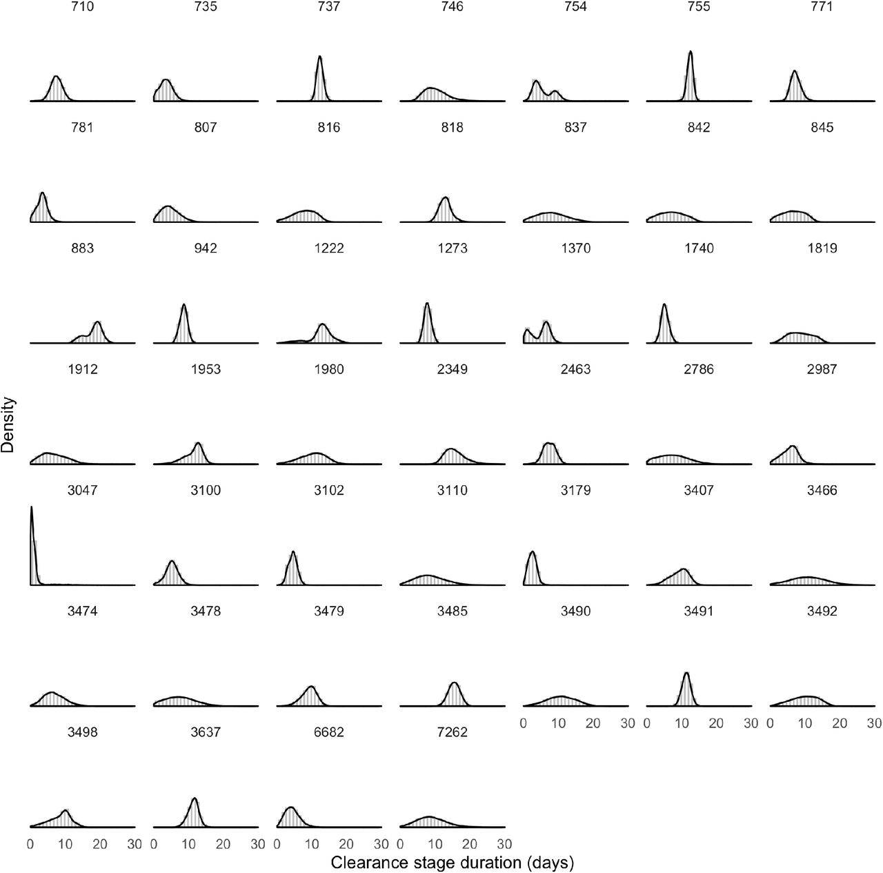

Thin grey lines depict 500 sampled trajectories. Points represent the observed data, with symptomatic individuals represented in red and asymptomatic individuals in blue.

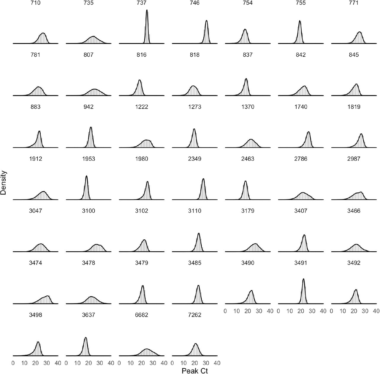
Histograms (grey bars) of 10,000 posterior draws from the distributions for peak Ct value (A), time from onset to peak (B), time from peak to recovery (C), and total duration of infection (D) across the 46 individuals with an acute infection. Grey curves are kernel density estimators to more clearly exhibit the shape of the histogram. Black curves represent the best-fit normal (A) or gamma (B, C, D) distributions to the histograms. The duration of infection is the sum of the time from onset to peak and the time from peak to recovery. The best-fit normal distribution to the posterior peak Ct value distribution had mean 22.3 and standard deviation 4.2; the best-fit gamma distribution to the proliferation stage duration had shape parameter 2.3 and inverse scale parameter 0.7; the best-fit gamma distribution to the clearance stage duration had shape parameter 2.4 and inverse scale parameter 0.3; and the best-fit gamma distribution to the total duration of infection had shape parameter 4.3 and inverse scale parameter 0.4.

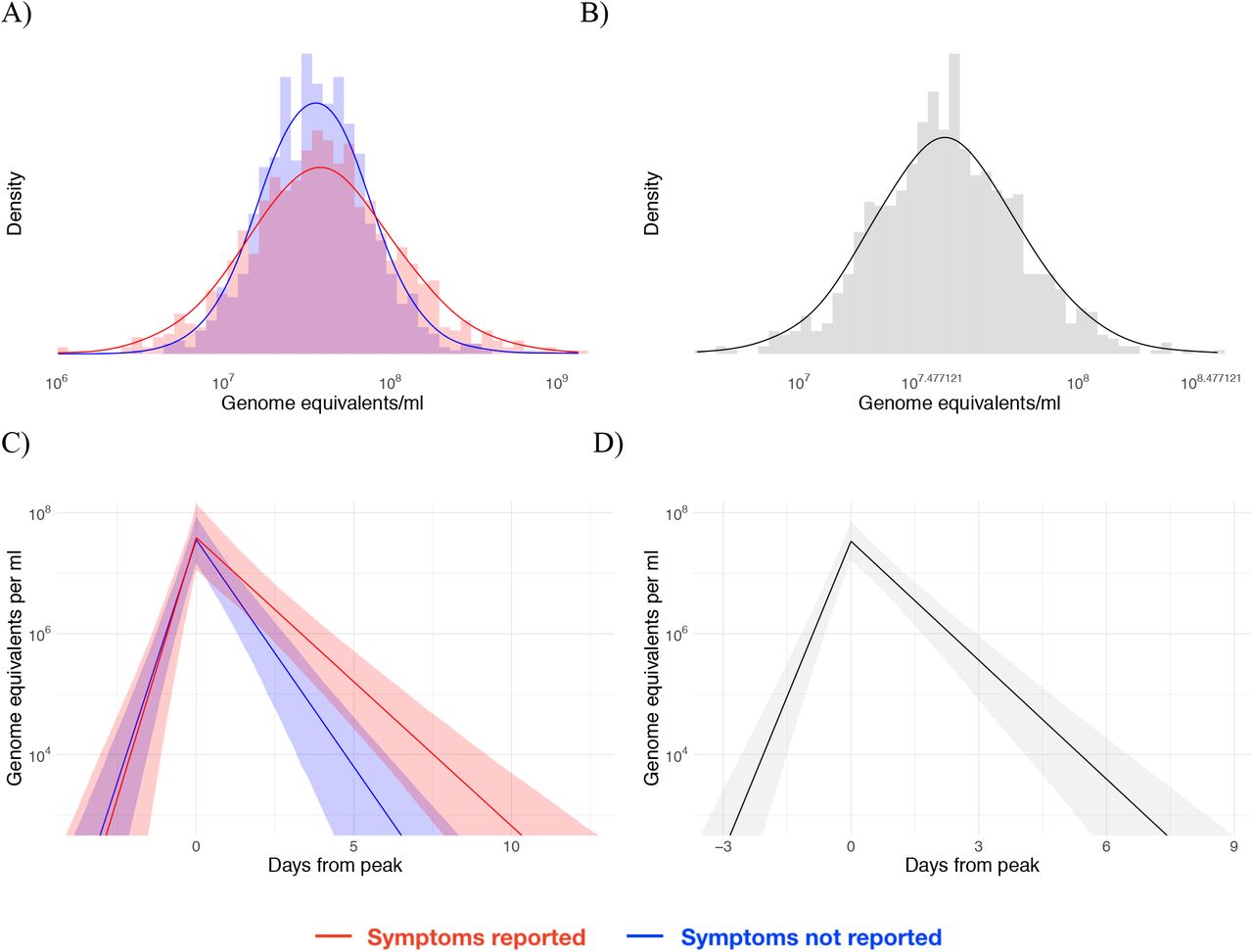
Posterior peak viral concentration distribution for symptomatic (red) and asymptomatic (blue) individuals (A) and for all individuals combined (B). Posterior viral concentration trajectory for symptomatic (red) and asymptomatic (blue) individuals (C) and for all individuals combined (D). The shaded bands in (C) and (D) represent 90% credible intervals for the trajectories.

Points depict the Ct values for SARS-CoV-2 nasal swab samples that were tested in both Florida and Yale labs. Ct values from Florida represent Target 1 (ORF1ab) on the Roche cobas system, and Ct values from Yale represent N1 in the Yale multiplex assay. The solid black line depicts the best-fit linear regression (intercept = –6.25, slope = 1.34, R2 = 0.86). The dashed black line marks the 1-1 line where the points would be expected to fall if the two labs were identical.

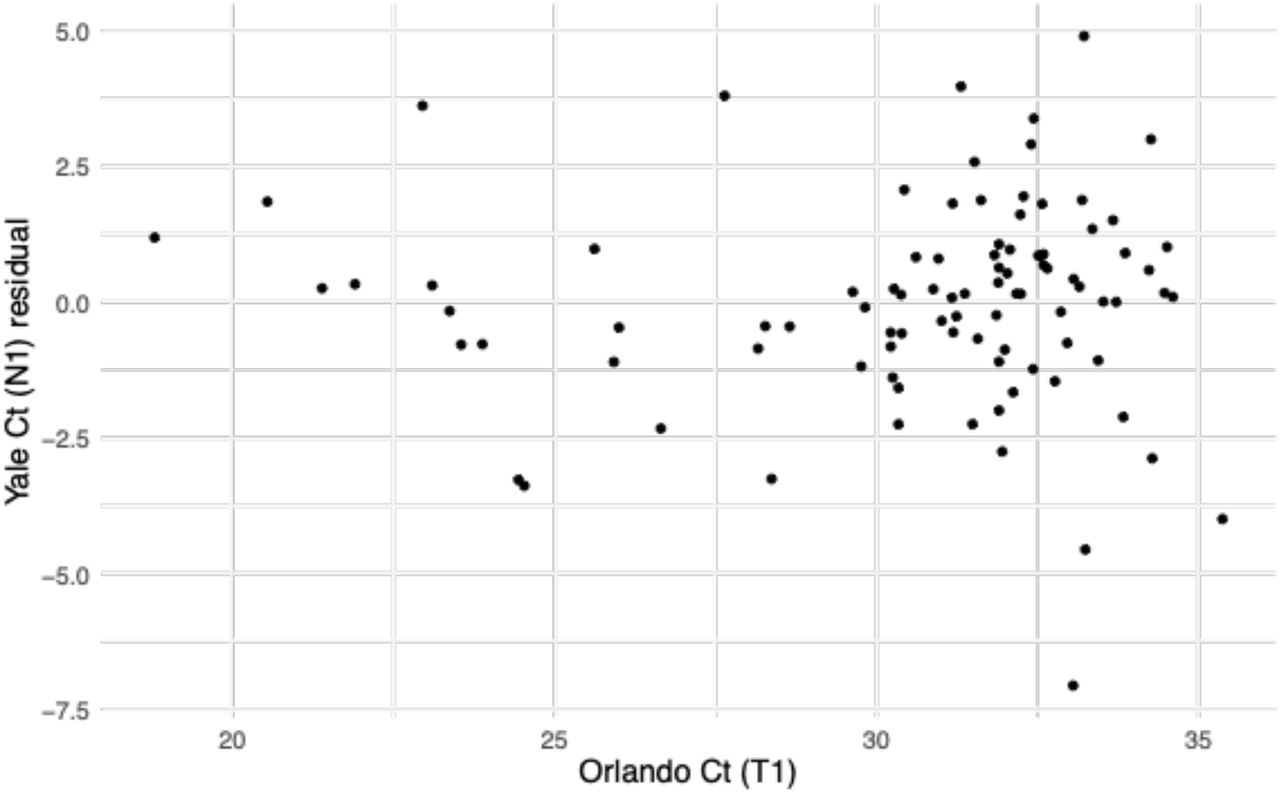
Points depict the residual after removing the best-fit linear trend in the relationship between the Yale and Florida Ct values.

The residuals were standardized (subtracted the mean and divided by the standard deviation) before comparing with the theoretical quantiles of a normal distribution with mean 0 and standard deviation 1. The points depict the empirical quantiles of the data points and the line depicts the where the points would be expected to fall if they were drawn from a standard normal distribution.

E[Ct] is the expected Ct value on a given day. The Ct begins at the limit of detection, then declines from the time of infection (to) to the peak at δ cycles below the limit of detection at time tp. The Ct then rises again to the limit of detection after tr days. The model incorporating these parameter values used to generate this piecewise curve is given in Equation S1 (Methods).
Acknowledgements
We thank the NBA, National Basketball Players Association (NBPA), and all of the study participants who are committed to applying what they learned from sports towards enhancing public health. In particular, we thank D. Weiss of the NBA for his continuous support and leadership. We are appreciative of the discussions from the COVID-19 Sports and Society Working Group. We also thank D. Larremore for comments on the manuscript, J. Hay and R. Niehus for suggestions on the statistical approach and P. Jack and S. Taylor for laboratory support.
Footnotes
↵† denotes co-senior authorship
Added section on effective sensitivity (Figure 4).


