
Abstract
Accurate estimates of the prevalence of infection are essential for evaluating and informing public health responses to the ongoing COVID-19 pandemic in the United States (US), but reliable, timely prevalence data based on representative population sampling are unavailable, and reported case and test positivity rates may provide strongly biased estimates. A single parameter semi-empirical model was developed, calibrated, and validated with prevalence predictions from two independent data-driven mathematical epidemiological models, each of which was separately validated using available cumulative infection estimates from recent state-wide serological testing in 6 states. The analysis shows that individually, reported case rates and test positivity rates may provide substantially biased estimates of COVID-19 prevalence and transmission trends in the U.S. However, the COVID-19 prevalence for U.S. states from March-July, 2020 is well approximated, with a 7-day lag, by the geometric mean of reported case and test positivity rates averaged over the previous 14 days. Predictions of this semi-empirical model are at least 10-fold more accurate than either test positivity or reported case rates alone, with accuracy that remains relatively constant across different US states and varying testing rates. The use of this simple and readily-available surrogate metric for COVID-19 prevalence, that is more accurate than test positivity and reported case rates and does not rely on mathematical modeling, may provide more reliable information for decision makers to make effective state-level decisions as to public health responses to the ongoing COVID-19 pandemic in the US.
Introduction
Accurate or reliable estimates of the prevalence of infection are essential for evaluating and informing public health responses to the ongoing COVID-19 pandemic. The gold standard method to empirically measure disease prevalence is to conduct periodic large-scale surveillance testing via random sampling 1. However, this approach may be time- and resource-intensive, and only a handful of such surveillance studies has been conducted so far in the United States (US) 2–4. Metrics such as the test positivity rate has been commonly used by public health officials to infer the level of COVID-19 transmission in a population and/or the adequacy of testing 5,6. The use of the test positivity rate for these purposes is often justified by referring to a WHO recommendation which was not necessarily intended to be used as such 7. In the absence of high-quality data and rigorous criteria for measuring COVID-19 prevalence and adequacy of testing, public health officials have relied on reported cases, test positivity rate, fatality rates, hospitalization rates, and epidemiological models’ predictions to inform COVID-19 responses. Reported cases and test positivity rate, though readily available and well-understood by public health officials, are very likely to substantially underestimate and overestimate, respectively, disease transmission/prevalence 1. Hospitalization and death rates are also similarly readily available, but tend to lag infections by several weeks and only reflect the most severe outcomes 1. Finally, epidemiological models are generally complex mathematical, computational, or statistical models that require extensive data and information for model training, and are perceived as a ‘black box’ by most public health practitioners and decision makers 8–10.
Here, we develop a simple semi-empirical model to estimate the prevalence of COVID-19 at the US state level based only on reported cases, test positivity rate, and testing rate. Specifically, we hypothesized that the preferential nature of diagnostic testing for individuals at higher risk of infection in the US is a convex function of the overall testing rate due to the “diminishing return” from expanding general population testing. We modeled this convexity using a negative power function, and calibrated the power parameter using prevalence predictions from two independent, data-driven epidemiological models 8,11,12 that were separately validated using available cumulative infection estimates from recent state-wide serological testing. Using this single fitted power parameter, we found that the state-level prevalence of COVID-19 in the US can be well-approximated by the geometric mean of the reported cases and test positivity rates. We evaluated how disease prevalence varies with changes in reported cases and test positivity, and the implications of applying this simple model on informing public health decision-making to the COVID-19 pandemic in the US.
Methods
Conceptual basis of a semi-empirical model for the prevalence of COVID-19 infection
Test positivity rate p+,τ (t) = N+,τ(t)/Ntest,τ(t) is defined as the percentage of positive diagnostic tests administered over a given period τ between t − τ and t. We first hypothesize that, because testing is currently “preferential” in that only those considered more likely to be infected due to symptoms, contacts, etc., are tested, p+,τ(t) is correlated to the lagged prevalence I(t − tlag)/N of COVID-19-infected persons in the population with a time-dependent bias parameter b(t):
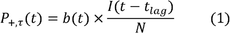
Conceptually, this relationship is shown in Figure 1A. We next hypothesize that the bias parameter b(t) is inversely related to the testing rate Λτ(t) = Ntest,τ(t)/N over the same period τ. Clearly, at a testing rate of 1, where everyone is tested, there is no bias, so b= 1. On the other hand, for very low testing rates, the bias is likely to be high, as only the most severely ill will be tested. For instance, if all COVID-19 deaths are tested daily, but no one else, then the bias will be equal to the inverse of the infected fatality rate (IFR), b = 1/IFR; and of course, in the limit of zero testing, the bias will be infinite. Moreover, at low testing rates, increasing the testing rate will likely preferentially increase the infected population testing rate relative to the general population testing rate, so b(t) will decline more rapidly than at higher testing rates, as there is “diminishing return” from increased testing. Thus, it is reasonable to assume that b(t) is a convex function of Λτ(t). We therefore model the bias as a negative power function of Λτ(t):
Conceptual model for relationship between test positivity, prevalence of infection, and testing rate. We assumed the test positivity rate is correlated to delayed disease prevalence with a bias parameter b(t). In A) the diagonal lines represent different values of the bias parameter and the U.S. state positivity rates from March-July are shown for reference. B) Illustrate the relationship between testing rate and bias parameter represented by equation (2). Here the shaded region represents different powers n ranging from 0.1 to 0.9, the dotted line represents n = 0.5, and the U.S. state testing rates from March-July are shown for reference.
Combining equations (1)-(2), and re-arranging leads to the following relationship between test positivity and the infectious population:

Additionally, because test positivity and the testing rate share a term Ntest,τ(t), equation (3) can be further rearranged as
 where the last term is the reported cases per capita C+,τ(t) = N+,τ(t)/N. Thus, our hypothesis predicts that the infectious population is proportional to a weighted geometric mean of the positivity rate and the reported case rate, with n = 1/2 corresponding to equal weighting.
We can also rearrange equation (1) and view the bias parameter as the relative efficacy of testing infected individuals compared to the general population:
Here,  is the daily rate of testing of infectious individuals (with averaging time τ and lag tlag), whereas Λτ(t) is the daily rate of testing of the general population, as previously defined. Thus, the bias reflects the extent to which infectious individuals are “preferentially” tested.
Fitting the power parameter of the semi-empirical model
For a given time point ti, we define the “effective” power parameter neff(ti) by solving equation (3) for n:
The positivity p+,τ(ti) and the testing rate Λτ(ti) are calculated from data obtained from the COVID Tracking Project 13, averaged of the past τ days. Because I is generally unobserved, we use estimates derived from data-driven epidemiological models. Two models of SARS-CoV-2 transmission in U.S. states are considered here: a Bayesian extended-SEIR model 12 (run through July 22, 2020) and a Bayesian semi-mechanistic model by Imperial College 14 (run through July 20, 2020), which applies the model published by Flaxman et al., 2020 8 to the US. These models are calibrated at the US state-level to reported deaths and/or cases, but do not utilize test positivity or testing rate as an input. Both of these are Bayesian models, so incorporate multi-parameter uncertainty, which is accounted for in our analysis by utilizing random samples of the posterior distributions for I.
The result of this procedure is a time-series in neff(ti), which we split approximately in half into a training set (ti ≤ May 31, 2020) and a validation set (ti ≥ June 1, 2020). Using intercept-only fixed and random effects linear models, we calculated the average power parameter with the training set, using an averaging time τ= 14 days and a lag tlag = 7 days. For fixed effects, a single power parameter was derived, whereas for random effects, state-specific power parameters were derived. We calculated the power parameter separately based on the extended-SEIR model only, the Imperial model only, and based on combining the two models (i.e., treating the two models as two independent measurements of I).
For each set of power parameter estimates, we evaluated predictive accuracy and precision for both the training set and the validation set by comparing the prevalence predicted using equation (4) to the predictions of the original epidemiological models. Specifically, the prediction errors (residuals) were calculated by comparison, after log10 transformation, to a random posterior sample from the extended-SEIR or Imperial model. Predictive accuracy was characterized by both the mean and median residual; predictive precision was characterized using both the usual root mean squared error (RMSE) 15, which assumes normally distributed errors, as well as the median absolute deviation (MAD), which is robust to outliers 16. Furthermore, the fraction of predictions within the posterior 95% Credible Interval (CrI) of the extended-SEIR or Imperial model (F95) as a metric of whether the semi-empirical-based model estimates of prevalence are consistent with the epidemiologic model-based estimates. These statistics were calculated for both overall as well as on a state-specific basis. For comparison, the same metrics for accuracy and precision were calculated based on reported cases or test positivity individually, as well as for the geometric mean of reported cases and positivity (corresponding to a power parameter n=1/2). Additionally, it should be noted that overall precision is limited by the posterior uncertainty of the original extended-SEIR and Imperial models, which had, respectively, RMSE of 0.19 and 0.09 and MAD of 0.18 and 0.10.
Epidemiological model validation
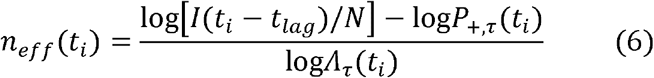
We independently validated the extended-SEIR and Imperial models by comparing their predictions to empirical data on the cumulative number of COVID-19 infections, which is available for 6 states, Connecticut (CT), Indiana (IN), Louisiana (LA), Missouri (MO), New York (NY), and Utah (UT), on a state-wise basis 2–4. For 4 states (CT, LA, MO, UT), data were downloaded from the Interactive Serology Dashboard for Commercial Laboratory Surveys 17. We only included data from states where the entire state was sampled or where adjustments for convenience sampling bias were integrated into the analysis.
Sensitivity Analyses
To assess the sensitivity of our results to the averaging time τ of 14 days, the time lag tlag of 7 days, and the split between training and validation data at May 31, 2020, we also considered an averaging time period τ of 7 days, time lag tlag of 0-14 days, and training data cutoffs of April 30 and June 30, 2020.
Software
All analyses were performed using the R statistical software (R version 3.6.1) in RStudio (Version 1.2.1335). Random effects models were fit using the lme4 package (version 1.1-21). We developed a publicly available online dashboard, using R and Shiny, to analyze and visualize state-level predictions of COVID-19 prevalence from our semi-empirical model. The dashboard self-updates once daily (https://wchiu.shinyapps.io/COVID-19-Prevalence-and-Trends-Alpha/).
Results
Validation of epidemiological model predictions
The comparison between epidemiological model predictions and empirical cumulative infections data are shown in Figure 2. For all states, the empirical data were consistent with the 95% CrI of the extended-SEIR model predictions. The Imperial model predictions were less consistent, with overprediction of CT and underprediction of NY and to some extent UT.
Validation of data-driven SEIR and Imperial epidemiological models using cumulative infections data.
Semi-empirical model calibration and predictions
The power parameter of the semi-empirical model was estimated by fitting equation (5) to the models’ predictions, resulting in a power parameter n ≈ 0.5, regardless of whether the estimate of the bias parameter was derived from the extended-SEIR, Imperial, or both models combined (Figure S1A). Similar parameter estimates were obtained when equation (5) was fitted to both training and validation data combined (Figure S1B). neff remained relatively constant over time, and the random effects estimate of neff remained close to the fixed effects estimate of ≈ 0.5 for nearly all states (Figure S2).
Given the power parameter, equation (4) was then used to predict the prevalence of infection based on the test positivity rate and reported case rates. We showed that the semi-empirical model predictions were consistent with those of the epidemiological models (Figures 3 & S3). Quantitative measures of accuracy and precision are summarized in Table 1 and Figure S4. The accuracy of the semi-empirical model, as measured by the mean and median residuals, ranged from −0.10 to 0.45 log-10 units, with the random effects estimate from the combined datasets having values of 0.07 and 0.04, respectively, corresponding to biases of < 20%. By comparison, mean or median residuals for reported cases and test positivity alone were < −1.17 and > 1.34, respectively, corresponding to biases of over 10-fold. The precision of the semi-empirical model over training and validation periods showed an overall MAD and RMSE in log-10 units ranging from 0.20-0.31 for the extended-SEIR model-based analysis, 0.16-0.28 for the Imperial model-based analysis, and 0.23-0.30 for the combined analysis (Figure S4). Precision for reported cases and test positivity were in the same range, with MAD and RMSE values from 0.2-0.3. The overall coverage F95 of the Imperial model was lower (0.3-0.8) as compared to the SEIR model (> 0.9), and uniformly zero for reported cases and test positivity (Table 1, Figure S4). The accuracy and precision were mostly similar for the fixed and random effects models (Figure S4). The simplified approach of using a geometric mean of test positivity and reported case rates to estimate prevalence was as accurate and precise as random effects models. Sensitivity analysis was conducted with different averaging times (7 or 14 days), lag times (1 to 14 days), and training data date range (t ≤ April 30, May 31, or June 30). Our results were shown to be robust for both epidemiological models (Figure S5).

Semi-empirical estimate of the infected population for each state, using random effects estimates for the power parameter estimated from both the extended-SEIR and Imperial-based datasets combined. Bands show the 95% CrI for the extended-SEIR and Imperial predictions.
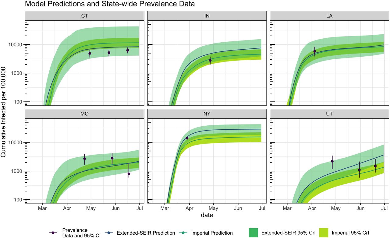
The pitfalls of relying on reported cases or test positivity rate alone to estimate the course of the epidemic are illustrated for four states, MN, MT, VA, and WI, where reported cases and positivity trends were in opposite directions in May and/or August (Figure 4). Specifically, in May, reported cases were rising substantially in MN, VA, and WI at the same time that the test positivity rate was declining, testing rate was increasing, and the model predicted prevalence was flat or decreasing (Figure 4). By contrast, in August, the states of MN, MT, and WI all showed declining reported case rates while positivity was increasing. Our model predicts that COVID-19 prevalence was either flat or increasing during this time. In both scenarios, the increase (decrease) in reported cases was due to expanded (declining) testing rates, respectively.
Examples of divergences between reported case rates and positivity rates for four states. For each state, the top panel is the prevalence as predicted by the semi-empirical model including a 7-day lag, whereas the bottom three panels show the reported case, positivity, and testing rates, each averaged over the last 14 days.
With our semi-empirical model, an individual state or municipality can easily utilize reported cases and positivity rates to better estimate their COVID-19 prevalence and its recent trend (Figure 5). We observed a positive correlation between state-level test positivity rate and reported cases (Figure 5A); however, states with the same reported case rate may differ greatly in their test positivity rates, resulting in substantial differences in prevalence. For example, thus was the case with DC and SD, which both had a reported case rate of ∼10 cases/100,000 on August 15, 2020, but a test positivity rate differing by almost 10-fold, resulting in a 3-fold difference in predicted prevalence. We showed that prevalence decreases (increases) when test positivity rate and reported case rate both decrease (increase), respectively (Figure 5B). However, when the trends in test positivity and reported cases are in opposite directions, the prevalence trend was shown to be highly dependent on the relative change in the value of the test positivity and reported case rates (Figure 5B).

A: Prevalence estimated for each state based on scatter plot of reported case rates and positivity rates. Prevalence increases to the upper right, and is expressed as a range to reflect the residual error estimated from the model. B: Two-week prevalence trend for each state, based on scatter plot of two-week changes in reported case rates and positivity rates. The shaded region expresses the uncertainty in the power parameter, and demarks where prevalence is predicted to be decreasing from where it is predicted to be increasing. C: Map of estimated prevalence and transmission trend. All rates are two-week averages evaluated on August 15, 2020, and all prevalence predictions are for a one-week lag.
Discussion
Reported case rates and test positivity rates have been widely used to inform or justify public health decisions as to increasing or relaxing intervention measures for the control of the COVID-19 pandemic in the US 18,19. A recent report of the National Academies of Sciences and Engineering Medicine (NASEM) has urged caution about the reliability/validity of directly using data such as reported case rates and test positivity rates to inform decision making for COVID-19 1. Though these data are, typically, readily available, the NASEM report concludes that they are likely to substantially underestimate or overestimate the real state of disease spread 1. It is therefore urgent and paramount to develop simple and more reliable data-driven metrics/approaches to inform public health decision-making.
We have developed a semi-empirical approach to estimate the prevalence of COVID-19 infections in a population using only reported cases and testing rates. Fitting only a single parameter, we find that the COVID-19 prevalence, with a 1-week lag, is well-approximated by the geometric mean of the positivity rate and the reported case rate averaged over the last 2 weeks. The prevalence predictions of our semi-empirical model were shown to compare favorably to those from two data-driven epidemiological models whose predictions were validated against U.S. state-level empirical data of COVID-19 prevalence. These predictions were at least 10-fold more accurate than estimates from using positivity or reported case rates alone. Although the prediction of our semi-empirical model has an uncertainty of about 3-fold in either direction, this degree of uncertainty is reduced by more than 10-fold compared to using positivity or reported case rates alone, and does not require developing and maintaining a complex data-driven mathematical model.
Our analysis suggests that public health policy on relaxing or reinstating of social distancing and other non-pharmaceutical interventions may be informed by available data in three main ways:
First, prevalence should be inferred as decreasing only if both reported cases and positivity rates are continuously declining without decreasing testing rates. This criterion can be taken as a surrogate for Reff(t) < 1, since declining prevalence is a sufficient condition for an effective reproduction number below one.
Two, the gap between reported case and test positivity rates, measured on the same scale (e.g., per 100,000), should be decreasing to ensure improvement in the sufficiency of testing. For most of the U.S., this gap has hovered around 1000-fold. For example, in MN, MT, VA, and WI (Figure 5), as testing ramped up in May, the gap narrowed; however, the gap widened in August, indicating that testing rates need to be brought back up. Indeed, as noted by the NASEM report, absolute testing rates, irrespective of positivity rates, may be a better indicator of the sufficiency of testing.
Finally, reported cases, test positivity, and testing rates should be publicly reported at the county or municipal level in order to provide local governments, health agencies, medical personnel, and the public with the necessary information to evaluate the local state of the pandemic. Currently, only reported cases are routinely provided at the local level, with positivity and testing rates comprehensively aggregated only at the state level.
As with any model, ours has a number of limitations. The most significant limitation is the reliance on epidemiologic model-based estimates of prevalence. However, we believe this concern is mitigated by our use of two independent estimates with completely different model structures, one of which is a more traditional extended-SEIR model, and other of which is a “semi-mechanistic” model partially statistical in nature. Moreover, both models were compared to the limited empirical prevalence data available. The other important limitation is the relatively limited range of test positivity rate and/or testing rate observations for most U.S. states. For this reason, we cannot necessarily guarantee that our results can be easily extrapolated to substantially higher testing rates (e.g., if wide-spread immunoassay-based testing were implemented). However, with higher testing rates, the difference between test positivity rates and reported case rates would decrease and reduce the effect of greater uncertainty in the degree of bias between the test positivity rate and the lagged prevalence. Finally, we did not address the sensitivity and specificity of diagnostic testing; however, the impact of imperfect test accuracy is likely to have a minimal impact on our results.
In conclusion, we found that the COVID-19 prevalence is well-approximated by the geometric mean of the positivity rate and the reported case rate. This predictor is 10-fold more accurate than either rate alone, and consistent with prevalence estimates from much more complex mathematical epidemiologic models. The use of this simple, reliable, and easy-to-communicate measure of COVID-19 prevalence will improve the ability to make public health decisions that effectively respond to the ongoing COVID-19 pandemic in the U.S.
Data Availability
The codes and data used to generate our results are available on GitHub
Funding
National Science Foundation (NSF DEB RAPID 2028632) and National Institutes of Health, National Institute of Environmental Health Sciences (P30 ES029067). The funders have no role in the design of the study, collection, analysis, and interpretation of data.
Conflict of Interest Disclosure
The authors declare no conflicts of interest
Ethical approval
Ethical approval was not required for this work.
Data sharing
The codes and data used to generate our results are available on GitHub at https://github.com/wachiuphd/COVID-19-US-Semi-Empirical


