
Abstract
Respiratory syncytial virus (RSV) causes a large burden of morbidity in young children and the elderly. Spatial variability in the timing of RSV epidemics provides an opportunity to probe the factors driving transmission of the virus, including factors that influence epidemic seeding and growth rates. Using hospitalization data from Connecticut, New Jersey, and New York, we estimated epidemic timing at the ZIP-code level using harmonic regression and then used a Bayesian meta-regression model to evaluate correlates of epidemic timing. Earlier epidemics were associated with larger household size and greater population density. Nearby localities had similar epidemic timing. Our results suggest RSV epidemics grow faster in areas with more local contact opportunities, and that epidemic spread follows a spatial diffusion process based on geographic proximity. Our findings can inform the timing of delivery of RSV extended half-life prophylaxis and maternal vaccines and guide future studies on the transmission dynamics of RSV.
Introduction
Respiratory syncytial virus (RSV) causes over 2 million outpatient visits annually among children in the United States (US) (1). It is one of the leading causes of hospitalization for lower respiratory infection among young children and the elderly (2, 3). Developing an effective vaccine against RSV is a high priority, as prophylaxis against RSV is prohibitively expensive and complicated to administer (4-7). The timing of the delivery of maternal RSV vaccines and extended half-life prophylaxis relies heavily on the timing of seasonal RSV epidemics. Understanding the community factors associated with the seasonality of RSV can help to optimize implementation of extended-life prophylaxis and maternal vaccines in the near future (8).
The timing of RSV epidemics varies markedly over space, both over large geographic scales and within a region (9, 10). Across the US, epidemics start earliest in the southeast and later spread to the north and west (11). Environmental and climatic drivers affect the timing of the seasonal epidemic by providing a favorable environment for the virus and by affecting host immune defense and/or behavior (e.g., indoor gatherings in the cold or rainy season) (12-14). However, while environmental factors can explain some of the broad spatial differences in the timing of RSV epidemics, they cannot fully explain finer-scale spatial variations (12, 15). At smaller spatial scales, epidemics tend to start earlier and last longer in urban areas than in surrounding suburbs and rural areas (7).
A number of factors can influence the timing of an RSV epidemic in a community. Epidemic timing is broadly determined by the growth rate of the epidemic and, if the virus does not persist year-round, by when the virus is re-introduced into the community (“epidemic seeding”) (Fig. S1). Epidemic growth rates affect the shape of the epidemic curve, while epidemic seeding influences when the epidemic starts. Growth rates can be influenced by a number of demographic factors, such as the population age distribution, susceptibility and contact rates (16) (Fig. S1). Contact rates are linked to factors like household size and population density (10, 17). Susceptibility to infection is linked to socioeconomic status (SES) (10, 17). Less is known about the factors that drive epidemic seeding for RSV. Research on other respiratory viruses has suggested that virus importation from surrounding areas, importation from other regions (e.g., transmission through long-distance air travel or commuting patterns), and transmission within and between schools may play a role in epidemic seeding (18-21).
In this study, we developed a Bayesian statistical model to probe the association between the timing of seasonal epidemics of RSV and potential explanatory factors that influence epidemic growth rates and seeding, including area-based measures of human mobility, demographic variables, geographic proximity, and school districts. The tri-state area that includes New York, New Jersey, and Connecticut is ideal to study the fine-scale spatial variation in RSV epidemics because of the demographic diversity, high volume of population movement, and relatively similar climate across the region. This area includes New York City, the most populous city in the US, as well as rural areas like the North Country region of New York state and Litchfield County in Connecticut. In addition, variation in community factors exist at small spatial scales (22). The strong commuting ties between New York City and surrounding areas offer valuable opportunities to compare the impacts of commuting flows and geographic distance on RSV epidemic patterns. This study aims to gain a better understanding of the factors influencing local epidemic timing.
Results
Characteristics of the model and data
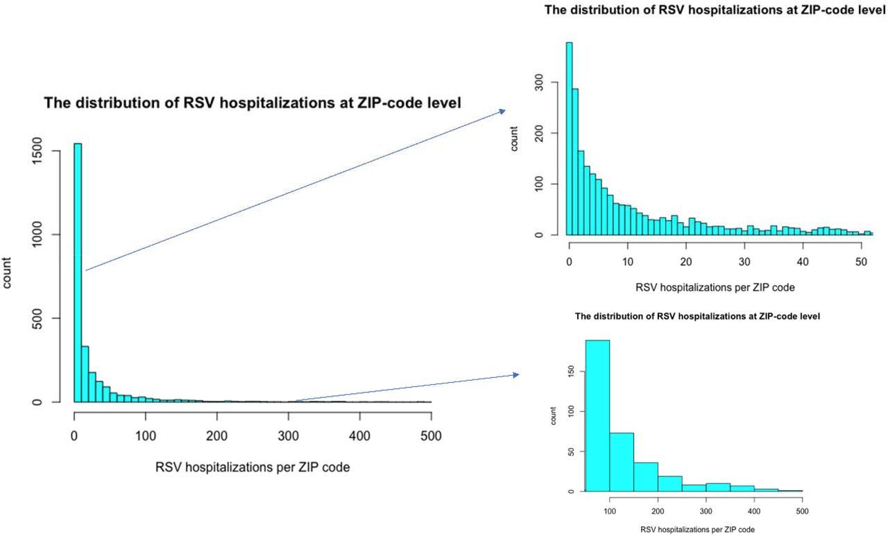
RSV-specific hospitalization data for children <2 years were obtained from State Inpatient Databases from the Connecticut Department of Public Health (CT-DPH) and the Healthcare Cost and Utilization Project maintained by the Agency for Healthcare Research and Quality (23). In total, the databases captured 67,244 RSV hospitalizations across 2,612 ZIP codes in New York, New Jersey, and Connecticut. The number of hospitalizations, commuters, and the length of study period varied among states (Table 1), as did the sociodemographic characteristics (Table S1, Fig. S2-S3).
Spatiotemporal pattern of RSV epidemics
RSV activity begins between late fall and early winter in the tri-state area (Fig. 1). The epidemics peaked between late winter and spring (Fig. 1). The estimated peak timing among ZIP codes ranged from late December to mid-March based on the best-fit model (Fig. 2). Visually, the local epidemics peaked earliest in urban areas (e.g., the New York metropolitan area) and then extended to less populous areas like upstate New York and eastern Connecticut. Epidemic peaks were generally earlier in New Jersey compared to the other states.

The solid color lines show the time series of RSV hospitalizations in children <2 years in Connecticut (CT), New Jersey (NJ), and New York (NY). The vertical dotted line indicates October of each year.

This model accounted for average household size, population density, population size, median income, school district, and geographic proximity. The study periods were July 1997 - June 2013 in Connecticut and July 2005 - June 2014 in New York and New Jersey.
Major correlates of local variation in RSV epidemic timing
We fit statistical models that included several demographic covariates while also characterizing the structure of the unexplained variability in the data (see Methods). Earlier epidemic timing was associated with higher population density in all three states (Table 2). There was an approximately 1.5-to 2-week difference in epidemic timing between the top and bottom deciles of population density. There was also an association between earlier epidemic timing and larger average household size in Connecticut and New York; the difference in epidemic timing between the bottom to top deciles of average household size was 0.7-1.3 weeks. In New Jersey, ZIP codes with higher income were associated with earlier epidemics. There was no association between the total number of people in the ZIP code and epidemic timing.
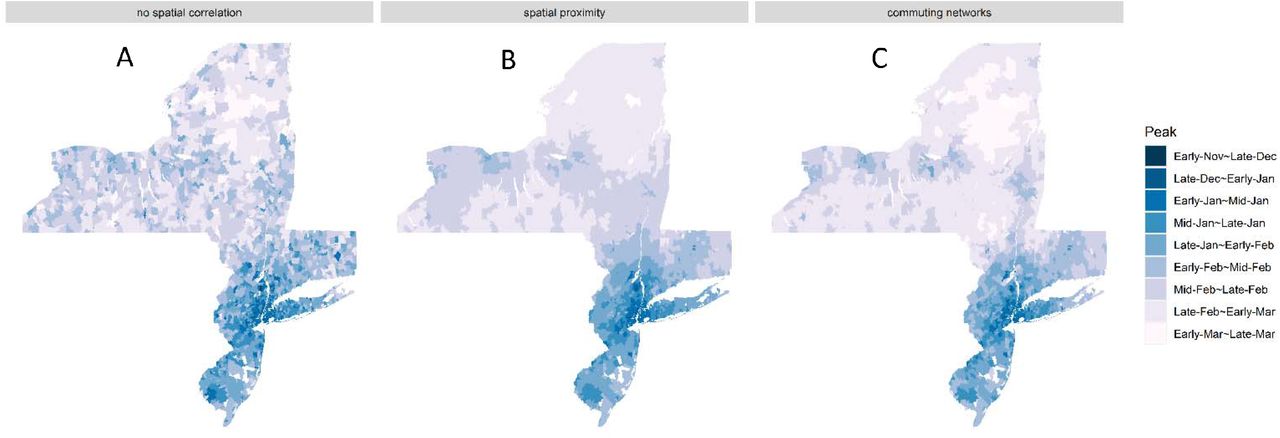
In all three states, there was substantial residual variability in the data after adjusting for the covariates. The covariates captured 41%, 30% and 51% of the variability in New Jersey, New York, and Connecticut, respectively. The best-fitting model assumed that the residual variation was correlated based on geographic proximity. Alternative models that assumed that the residual variation was related to commuter connectivity or that assumed no spatial structure fit less well (Table 3). In Connecticut, the geographic proximity model only fit marginally better than the commuting model. The residual variability in the geographic proximity model was further partitioned into variation based on geographic adjacency and variability based on school district boundaries. Geographic adjacency explained 89%, 94% and 69% of the total residual variability in New Jersey, New York, and Connecticut, respectively. School district effects contributed relatively little to the variations in epidemic timing (Table 4). The proportion of variability explained by population density, household size, school districts, and adjacency varied between states; however, their relative importance was consistent across states (Table 2 and Table 4).
Posterior means and 95% credible intervals are displayed.
Discussion
Understanding the timing of RSV epidemics is essential for certain interventions against RSV, including the administration of prophylactic antibodies and for assessing when to immunize pregnant women. We sought to better understand the underlying community factors associated with the timing of RSV epidemics. We find that the timing of RSV epidemics is highly spatially structured and demonstrate considerable variation, beginning in large urban areas and radially spreading to rural places over a 2.7-month period in the tri-state area. Epidemics generally peaked earlier in ZIP codes with higher population density and larger average household size, and epidemic timing in one location was correlated with timing in neighboring areas.
The covariates that were most strongly associated with earlier epidemic timing (population density and household size) could be related to the frequency of contact opportunities that lead to transmission (Fig. S1). Frequent contacts lead to rapid viral spread and epidemic growth, consistent with a positive correlation between population density and estimated RSV transmission rates for different US states (12). The strong connectivity between neighboring areas could reflect epidemic seeding (Fig. S1). Having stronger connections between proximate communities could provide more opportunities for introduction of the virus, eventually forming successful local chains of infection (24). This is supported by the localized and radially diffusive epidemic pattern. Other factors, such as gathering within schools and commuter flows, might also contribute to RSV transmission, but our analyses suggest these are not the major drivers of the observed spatial patterns in this population.
By mid-January, the tri-state area is usually well into its annual RSV season, but so far in late January 2021, the level of RSV activity remains low (25). The positivity rate of RSV detection in this area has declined since non-pharmaceutical interventions (NPIs) to mitigate the COVID-19 pandemic, such as travel bans, mask wearing and social distancing, were introduced in March 2020 (25). The measures taken to slow COVID-19 transmission are likely also effective in controlling RSV epidemics. Studies in Western Australia found that RSV in children dropped 98% through their winter of 2020, even though schools were open (26). This natural experiment suggests that gathering within schools may not be the major driver of RSV epidemics (or at least is not sufficient in light of other measures).
We found that higher median income is associated with earlier epidemics in New Jersey but not in the other states. The positive correlation between median income and the observed RSV epidemic timing in New Jersey could reflect a greater delay between infection and hospitalization in poorer neighborhoods (Fig. S1). It is also possible that the lack of an association in Connecticut and New York may result from the bidirectional effect of socioeconomic status on RSV epidemic timing. Low socioeconomic status may also increase susceptibility to RSV, thereby increasing the epidemic growth rate, although this effect may be partially mediated through differences in household size (Fig. S1).
The results from our study have important implications for planning clinical trials and developing transmission dynamic models for RSV. First, since household size may be associated with the risk of exposure and transmission of RSV, vaccine trials should ensure that household size is balanced between vaccinees and non-vaccinees. Second, transmission dynamic models should account for spatial heterogeneity as well as spatial correlations in the force of infection (e.g., using a meta-population model). The spatial patterns of RSV epidemic timing from the best-fit model show considerable discrepancies between urban and rural areas, highlighting the need to consider these as distinct spatial units in RSV transmission models.
Our findings are consistent with previous genomic analyses of RSV, which found that household transmission is common, and viruses from nearby households share similar phylogenetic origins (27, 28). However, due to the small sample size and study design, genomic analyses were unable to compare the different transmission environments and their relative role in local RSV transmission (27, 28). Using empirical epidemiologic, demographic and commuting flow data, our research has found evidence to fill this knowledge gap. Previous epidemiological studies also suggested that household crowding and/or a larger number of siblings are associated with increased risk of severe RSV lower respiratory tract infection (17). These findings together provide a more complete picture of the major drivers of RSV transmission and how local risk factors affect regional patterns of RSV epidemic spread.
Other factors might also contribute to RSV spatial transmission and local seasonality (Fig. S1). There are limits to what can be mechanistically tested with the statistical model we used in this study. As the demographic variables tested in our model may represent other underlying mechanisms, it is difficult to pinpoint the exact drivers of RSV dynamics with great certainty. For example, our results will not be able to confirm who drives transmission within households, as household size is correlated with the share of school-age children per household and the probability of having very young children. Mechanistic transmission dynamic models (e.g., meta-population models) that explicitly capture transmission and host immunity are needed to further study these issues.
Notably, the spatial spread pattern of RSV epidemics differs from that of influenza (21, 24, 29), which suggest different age groups drive transmission of RSV and influenza (16). As a result, the level of indirect protection that might be generated by vaccinating different age groups is expect to vary for the two pathogens (30, 31). Spatial studies suggested that commuting flows drive the spread of seasonal influenza epidemics, while school-age children may have been major drivers of the 2009 H1N1 pandemic in the US (21, 24, 29). However, our analysis suggests that short-range modes of transmission, especially transmission within and between local communities, predominates for RSV. This, together with the fact that children under five have the highest overall risk of RSV infection (16), suggests that it is possible that infants and pre-school aged children drive RSV transmission. This could potentially be explained by the build-up of partial immunity against RSV due to previous exposure as age increases (32).
Our study and interpretations have several caveats. First, we performed an ecological analysis with aggregate data on sociodemographic characteristics at the ZIP-code level. Thus, we did not assess the role of individual household size on risk of RSV transmission. Likewise, there could be substantial heterogeneity within ZIP codes in the demographic characteristics that we evaluated. Second, the aggregation of ZIP-code level cases to dominant school districts may have led to some misclassification and does not account for the multiple primary schools typically found within a school district. This could have affected the data-fitting process and resulted in a lower percentage of variability that was explained by school districts. However, since school calendars and school bus routes are shared within the same school district, using school districts can help us evaluate the transmission within and between schools. Third, monthly time series may disguise some detailed variation compared to weekly time series. However, in a sensitivity analysis, we estimated the peak epidemic timing in Connecticut using both weekly data and data aggregated to the monthly level and found that the phase estimates were nearly identical. Thus, the availability of finely-resolved temporal surveillance data is not essential to capture broad patterns in epidemic timing. Fourth, while we draw inference about the potential mechanisms that drive RSV transmission, the pattern of spatial diffusion that we observed may result from a wide range of possibilities. Thus, the interpretation of our study results needs to be further explored with epidemiologic studies, genomic analyses, and transmission dynamic models. More detailed data, such as the proportion of young children attending daycare in each ZIP code, could help to address remaining gaps in the knowledge of this system.
In conclusion, our results reveal significant variation in local RSV epidemic timing. We find evidence that the timing of RSV epidemics is associated with average household size, population density, median income, and epidemic timing in neighboring areas. In general, RSV epidemics take off earlier in urban areas and spread to rural places with low population density and average household size. These findings highlight the need for infection control within households and communities to protect high-risk populations. Our results also offer additional insights that can be used to inform the development of transmission dynamic models and provide guidance on future vaccine target populations and clinical trial design.
Materials and Methods
Data source
RSV-specific hospitalization data for children <2 years from 1997 to 2013 were obtained from the Connecticut State Inpatient Database through the Connecticut Department of Public Health (CT-DPH). This dataset included the week and month of admission and the ZIP code of residence. Similar data for New York state and New Jersey were obtained from State Inpatient Databases of the Healthcare Cost and Utilization Project maintained by the Agency for Healthcare Research and Quality; these comprehensive databases contain all hospital discharge records from community hospitals in participating states (23). Datasets include the month of hospitalization (for 2005-2014) and ZIP code of residence. Cases were defined as any child <2 years old whose hospital discharge diagnostic codes included 079.6 (RSV), 466.11 (bronchiolitis due to RSV), or 480.1 (pneumonia due to RSV), based on the International Classification of Disease Ninth Revision [ICD-9]. The analysis of the data was approved by the Human Investigation Committees at Yale University and the CT-DPH. The authors assume full responsibility for analyses and interpretation of data obtained from the CT-DPH.
Geospatial data at the ZIP-code level were obtained from the US Census Bureau’s Geography program (33). Information about population size <5 years old, average family type of household size and median income in each ZIP code area were obtained from the US Census Bureau’s American Community Survey (34-36). School district information was obtained from state geographic information systems, education department databases, and national center for education statistics (37-40). Countrywide commuting patterns at the ZIP-code level were obtained from the US Census Bureau’s Center of Economic Studies (41). All geographic and demographic data except median income are from the 2010 census, since annual inter-censual estimates were not available for all variables during this time period; this corresponds to the midpoint of the hospitalization data from New York and New Jersey. We also performed sensitivity analyses using data from 2000 in Connecticut and 2014 in New Jersey to evaluate whether changes in demographic variables would influence the estimates. Ideally, we would perform sensitivity analysis using covariate data from each year in each state; however, due to the computational cost, we chose to perform sensitivity analysis using the data from two ends of the time-series spectrum.
Model structures
Two-stage hierarchical Bayesian model
We estimated the factors associated with spatial variability in the timing of RSV epidemics at the ZIP-code level using a two-stage modeling approach. In the first stage, we obtained an estimate of epidemic timing (phase shift) for each ZIP code, and a corresponding measure of uncertainty, using harmonic regression. In the second stage, we fit hierarchical Bayesian spatial models with multiple covariates and different correlation structures. Model comparison techniques were used to evaluate the different models.
First stage model
The first stage consists of a harmonic Poisson regression model that estimates the amplitude and phase of seasonal RSV epidemics (18). This model was fit separately to the monthly time series of observed RSV hospitalizations from each ZIP code and was specified as:
The observed number of RSV cases in ZIP code i during month t is denoted as Yit, phase Ti captures the shift in peak timing (with the 12-month period starting in early July), is ξi the amplitude of seasonal epidemics, ln(pop5i) is the offset term for the population under 5, αi is the intercept, and φit is an observation-level random effect that accounts for any unexplained variability in the data (i.e., overdispersion). In this first stage, all model parameters were estimated separately for each ZIP code. This model was fitted in the Bayesian setting using the rjags package with weakly informative prior distributions specified for all model parameters (42). Full details are provided in the Supplement.
Second stage model
Based on estimates of Ti (posterior means) and their uncertainty (posterior standard deviations) obtained from the first stage, we used a Bayesian meta-regression approach in the second stage to explain spatial variability in the epidemic peak timing of RSV (43-47). Specifically, we first transformed the peak timing parameters, whose values are confined to [0, 2π], to have support on the real line (useful for the second stage regression modeling) such that  . Next, we obtained posterior means,
  , and posterior standard deviations,
 , from the first stage and specify the second stage model as
  where
where  . We used stepwise forward selection to choose candidate variables from the causal diagram for use in our second stage models (Fig. S1). We performed variable selection using a simplified version of the regression model that excluded the spatial random effects. We began with the two variables (average household size and population density) that decreased the residual variance the most. We then included the variables representing other mechanisms, provided they did not affect the posterior estimates of the previously selected variables to avoid issues related to multicollinearity.
We evaluated several alternative correlation structures to describe the residual variation in the data after adjusting for the ZIP-code level covariates (average household size, population density, population size, and median income). All covariates were standardized before entering the models. The structure of the second stage model was specified as:
 where ηd(i) and ϕi are random effects for school district d and ZIP code i. The school district random effects are distributed as
  , where d(i) is the school district that includes ZIP code i. The alternative structures for ϕi were:
No residual spatial correlation in RSV epidemic timing:
 .
.RSV epidemics have similar timing in neighboring geographic locations:
(43). Here, spatial proximity was defined by ZIP codes with adjacent borders.RSV epidemics have similar timing in locations connected strongly by commuting patterns:
(43). Here, spatial proximity was defined by commuting patterns across ZIP codes.
We estimated the proportion of residual variability explained by the spatially correlated random effects (ϕi) versus the school district random effects (ηd(i)) (see Supplement). We also calculated the difference in epidemic timing between the top and bottom deciles for each variable to measure the relative importance of input variables (see Supplement). More details about hyperprior distributions for these different models are given in the Supplement.
Parameter estimation was carried out separately for each of the three states via Markov chain Monte Carlo simulation with an initial burn-in period of 10,000 iterations and a subsequent set of 50,000 posterior samples collected for all parameters in the first stage (48). A burn-in of 5,000 iterations and a subsequent set of 20,000 posterior samples were collected in the second stage. Convergence was assessed by Gelman-Robin diagnostics and examining individual parameter trace plots, with no obvious signs of non-convergence observed. Deviance information criterion (DIC) was calculated for each model to compare the performance; a lower DIC indicates a model has an improved balance of fit and complexity (49). Equations for the calculation of residual variance can be found in the Supplement. All analyses were performed using R v3.5.3.
Data Availability
The demographic and geographic data that support the findings of this study are available in the Geography program of the US Census Bureau, the American Community Survey of the US Census Bureau, the Center of Economic Studies of the US Census Bureau, state geographic information system, and education department databases. The hospitalization data are not available publicly but can be attained from the State Inpatient Database with the permission of the Connecticut Department of Public Health (CT-DPH) and upon signing a data use agreement with the Agency for Healthcare Research and Quality.
https://www2.census.gov/geo/tiger/TIGER2010/ZCTA5/2010/
https://data.census.gov/cedsci/
https://njogis-newjersey.opendata.arcgis.com/datasets/ca144194df66491d83b8f8bf338e0172_2
https://gis.ny.gov/gisdata/inventories/details.cfm?DSID=1326
http://magic.lib.uconn.edu/connecticut_data.html
Funding
DMW, VEP, JLW acknowledge support from grant R01AI137093 from the National Institute of Allergy and Infectious Diseases/National Institutes of Health. ZZ acknowledges support from the China Scholarship Council (CSC) scholarship #201806380027. The content is solely the responsibility of the authors.
Author contributions
ZZ implemented the study, analyzed the data and drafted the article. DMW conceptualized and designed the study. VEP helped revise the study design and manuscript for important intellectual content. JLW designed the study’s analytic strategy and helped prepare the Methods sections of the text.
Competing interests
VEP has received reimbursement from Merck and Pfizer for travel expenses to Scientific Input Engagements on respiratory syncytial virus. DMW has received consulting fees from Pfizer, Merck, GSK, and Affinivax for topics unrelated to this manuscript and is Principal Investigator on a research grant from Pfizer on an unrelated topic. All other authors report no relevant conflicts.
Data and materials availability
The demographic and geographic data that support the findings of this study are publicly available from the Geography program of the US Census Bureau, the American Community Survey of the US Census Bureau, the Center of Economic Studies of the US Census Bureau, National Center for Education Statistics, state geographic information system, and education department databases. The hospitalization data are not available publicly, but can be obtained from the State Inpatient Database with the permission of the Connecticut Department of Public Health (CT-DPH) and upon signing a data use agreement with the Agency for Healthcare Research and Quality. The R code for this study can be found in the GitHub repository: https://github.com/weinbergerlab/RSV_spatiotemporal.
Supplementary Materials
Supplementary Materials and Methods
Two-stage model to estimate epidemic peak timing
First Stage
The priors of the first stage model were as follows:
Second Stage
The priors of the coefficients of the input variables were:
The prior of the variance  of the school district random effects ηd(i) was:
The details of the structures of ϕi and the corresponding priors for the alternative versions of ϕi were:
(1) Version 1
Assumes there is no spatial correlation in RSV epidemic timing within the three states after adjusting for ZIP code-level covariates and shared variability within school districts. In order to obtain desired levels of statistical precision and avoid extreme rates based on small local sample sizes, the non-spatial model uses an i.i.d. random intercept to pool information across all small areas, then the model pulls estimates toward a global mean without regard to their relative spatial locations. The priors of this structure were as follows:
 The model variables are defined as:
ϕi: ZIP-code-level random effect
- : variance of ZIP code random effect

(2) Version 2
Assumes that RSV epidemics have similar timing in neighboring geographic locations after adjusting for ZIP-code-level covariates and shared variability within the same school district. In this structure, we adopted a conditional autoregressive (CAR) prior model with a Leroux formulation for smoothing the spatial random effect term, which allowed the models to have a single random intercept accounting for both spatially structured and unstructured variation (43). The degree of smoothing in spatial and non-spatial components of the random effect was determined by the empirical data. Spatial correlation was estimated by ρ. The neighborhood matrix contained information about spatial proximity between two locations. Here, spatial proximity was defined as ZIP codes with adjacent borders. The model is given as:
n: total number of ZIP code areas.
wij: equal to one if regions i and j share a common border, equal to zero otherwise (wii = 0 for all i).
ρ: spatial autocorrelation parameter; ρ ∈ [0,1), where ρ = 0 corresponds to spatial independence, simplifying the model to an independent random effects model, and ρ near 1 means strong spatial autocorrelation. However, ρ should not equal to 1, since this corresponds to an improper intrinsic autoregressive (IAR) model(44, 47).
- : variance of spatial proximity random effect.

(3) Version 3
Assumes RSV epidemic timing is explained by commuting flows after adjusting for ZIP-code-level covariates and school districts. The model structure was similar to the second hypothesis, but instead of defining the neighborhood matrix based on shared geographic borders, spatial proximity in the commuting model (W) was defined by the frequency of commuters between two locations. The overall model structure was the same as the model structure of the geographic proximity model. The only difference is the definition of matrix which is given as:
 where i ∼ j suggests that there are more than 5 commuters between ZIP codes i and j; the element v ij is defined by the maximum commuting frequency between ZIP codes i and j.
We used the following equations to calculate the percentage of variability in RSV epidemic timing explained by the various components of the best-fit model:
Percentage of variability explained by fixed effects
- : variance of school district effect in the spatial correlated model with fixed effects
- : variance of spatial proximity random effect in the spatial correlated model with fixed effects
- : variance of school district effect in the spatial correlated model without fixed effects
- : variance of spatial proximity random effect in the spatial correlated model without fixed effects


Percentage of variability explained by school district
Percentage of variability explained by spatial proximity
The difference in epidemic timing between the top and bottom decile for each variable (in months) was calculated as:
School District Interpolation
RSV hospitalizations were reported at the ZIP-code level. We applied an areal interpolation process to derive estimates at the school-district level from the ZIP-code level data. First, we calculated the intersection between ZIP codes and school districts. Then we measured their areal weight and multiplied the value by the weight to get an estimate of hospitalizations for each intersection. We then aggregated these estimated values to get an estimate for each school district (50). The analysis was performed using the areal package version 0.1.6 (51).
Supplementary Figures
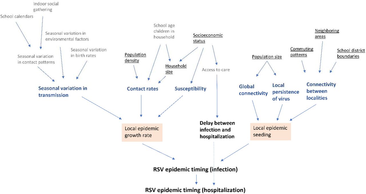
There are three levels of factors that influence the RSV epidemic timing. The most direct factors are highlighted in the first level. The factors that may contribute to epidemic growth and epidemic seeding are in the second level with bold font. The third level is the individual variables that affect the factors in the second level. We underlined the third-level factors that are included in our analysis. The reasons for choosing these factors are as follows:
While school calendars are likely important, school start dates do not vary widely across this region and so are unlikely to affect the timing of seasonal RSV epidemics. We also did not include environmental factors because we consider finer-scale spatial variation. Seasonal variation in birth rates could influence the size of susceptible populations in the RSV season. However, we did not have this information available at the monthly ZIP-code level. The share of school-age children in a household may affect possible importation of RSV into the household from schools, but its effect was non-significant in models that also included household size, and it is essentially capturing the same underlying process: that higher contact opportunities lead to rapid epidemic growth. Therefore, we only included the household size as a covariate. We examined the correlation with the remaining covariates and included all available factors.

The cut-off point for the subunit plots is 50 RSV hospitalizations in a ZIP code.
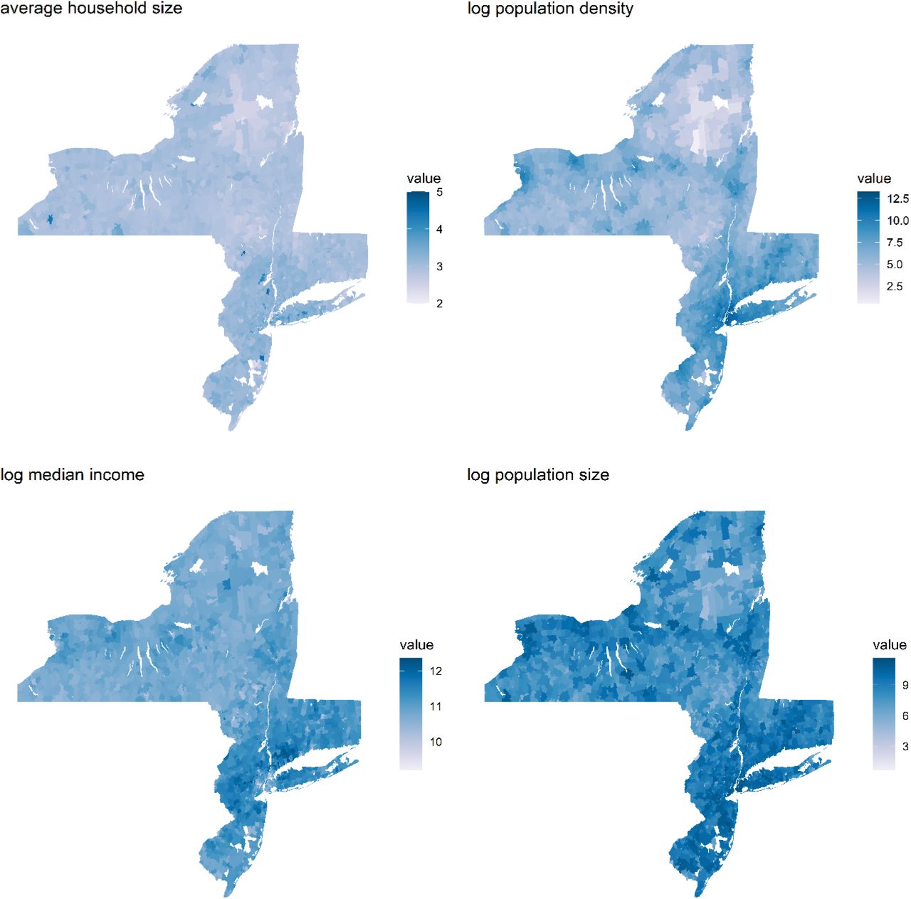
The color bars are used to indicate the value of the covariate in each ZIP code, with darker colors indicating higher values. The white spots in the map are locations that are not associated with RSV hospitalizations such as water bodies, forests and large facilities.

(A) No spatial correlation: This model assumed no spatial correlation while accounting for average household size, population density, population size, median income, and school district. (B) The best-fit model: This model accounted for average household size, population density, population size, median income, school district, and geographic proximity. (C) Commuting network model: This model accounted for average household size, population density, population size, median income, school district, and commuting flows. The study periods are July 1997 - June 2013 in Connecticut and July 2005 - June 2014 in New York and New Jersey.

In the Stage One panel, the left panel shows the estimated RSV epidemic peak timing and the right panel shows the log-precision of the first stage model. In the Stage Two panel, from left to right are the precision after log transform of the model that assumed no spatial correlation, the spatial proximity model, and the commuting network model, respectively. Darker colors indicate greater precision in the estimated values. Before applying the second stage model, estimates of peak timing from the first stage model were more variable overall, including a few extreme values. The estimates of many ZIP codes had low precision in the stage one model. The geographic-distance-based spatial correlation structure pooled information across nearby small areas, obtaining desired levels of statistical precision and avoiding extreme values based on small local sample sizes.

The left panel shows the model predictions of epidemic peak timing from the spatial proximity model and the right panel shows the predictions for the fitted model based only on the fixed effects (random effects held to 0).
Supplementary Tables
Descriptive statistics and sociodemographic factors by ZIP code in New Jersey, New York, and Connecticut, 2010.
Additional Analyses
Sensitivity Analysis on Time Series Data
To examine the robustness of our analysis, we compared the phase estimates from models fitted to monthly aggregated data to the phase estimates from models fitted to weekly data in Connecticut. We aggregated the original weekly time series data in Connecticut to the monthly level based on the month that the first dates of the week fell into. We then ran the hierarchical Bayesian model without covariates and spatial structures twice with the two types of data. We then measured their similarity by constructing a linear regression and calculating the slope and intercept (Figure S7).

The regression coefficient 1.04 showed that phase estimates based on models fitted to aggregated monthly data are consistent with those estimated using weekly data.
Sensitivity Analysis on Socio-demographic Data
We also ran our models using the socio-demographic data from 2000 in Connecticut and 2014 in New Jersey as covariates to ensure the associations observed are robust to potential changes in socio-demographics over time. Due to the lack of data on commuting patterns before 2002, we only tested the relative importance of spatial structure based on the commuting data from 2002 in Connecticut and 2014 in New Jersey. These data covered most of the time period of our study.
The DIC scores in both sensitivity analyses were lowest for the model that assumed a spatial correlation defined by neighboring areas (Table S3), which is consistent with our main findings. The results of standardized coefficient analyses and percentage of random effects explained by spatial proximity showed similar patterns in the sensitivity analysis and our main analysis (Table S4). The fixed effects explained 41% of the total variability in New Jersey and 59% in Connecticut (Table S5). Overall, the choice of socio-demographic data and commuting patterns did not affect the conclusions of our study.
DIC scores of competing models fitted to RSV hospitalizations in New Jersey and Connecticut using socio-demographic data from 2014 (New Jersey) and 2000 (Connecticut).
Posterior estimates of standardized fixed-effect coefficients for models fitted to RSV hospitalizations in New Jersey and Connecticut using socio-demographic data from 2014 (New Jersey) and 2000 (Connecticut) versus data from 2010.
Percent of residual variation attributable to each random effect for models fitted to RSV hospitalizations in New Jersey and Connecticut using socio-demographic data from 2014 (New Jersey) and 2000 (Connecticut). Posterior means and 95% credible intervals are displayed.
Acknowledgments
Footnotes
Revised based on Reviewers comments.
References


