
Abstract
The frequently stated goal of COVID-19 control is to “flatten the curve”; that is, to slow the epidemic by limiting contacts between infectious and susceptible individuals, and to reduce and delay peak numbers of cases and deaths. Here we investigate how the scale and dynamics of COVID-19 epidemics differ among 26 European countries in which the numbers of reported deaths varied more than 100-fold. Under lockdown, countries reporting fewer deaths in total also had lower peak death rates, as expected, but shorter rather than longer periods of epidemic growth. This empirical analysis highlights the benefits of intervening early to curtail COVID-19 epidemics: the cumulative number of deaths reported in each country by 20 June was 60-200 times the number reported by the date of lockdown.
One-sentence summary The COVID-19 death toll has varied more than 100-fold across European countries; the total number of deaths reported in each country was 60-200 times the number reported by the date of lockdown.
Main text
Physical distancing flattens an epidemic curve by reducing the contact rate between infectious and susceptible individuals. A lower contact rate lowers the basic case reproduction number, R0, which reduces peak incidence and death rates and distributes the burden of illness over a longer time period (1–4). Flattening the curve protects health and health services.
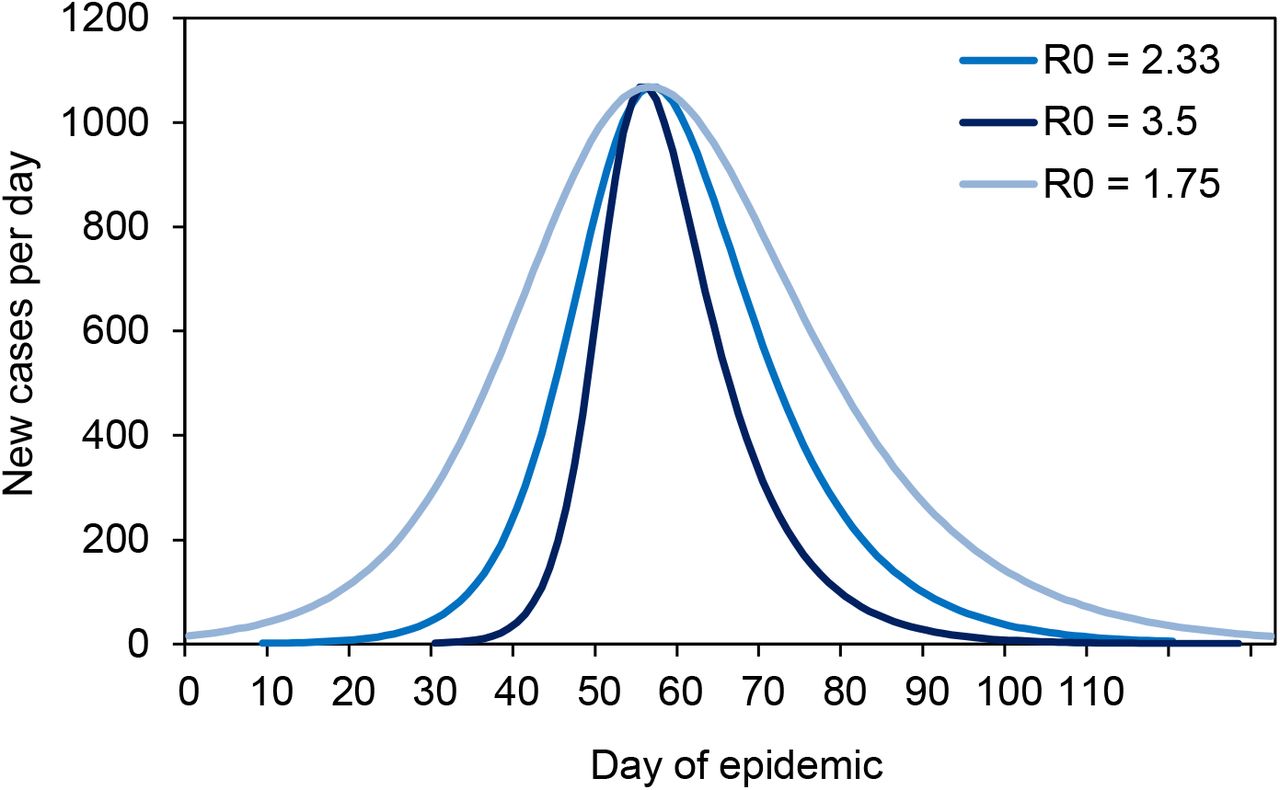
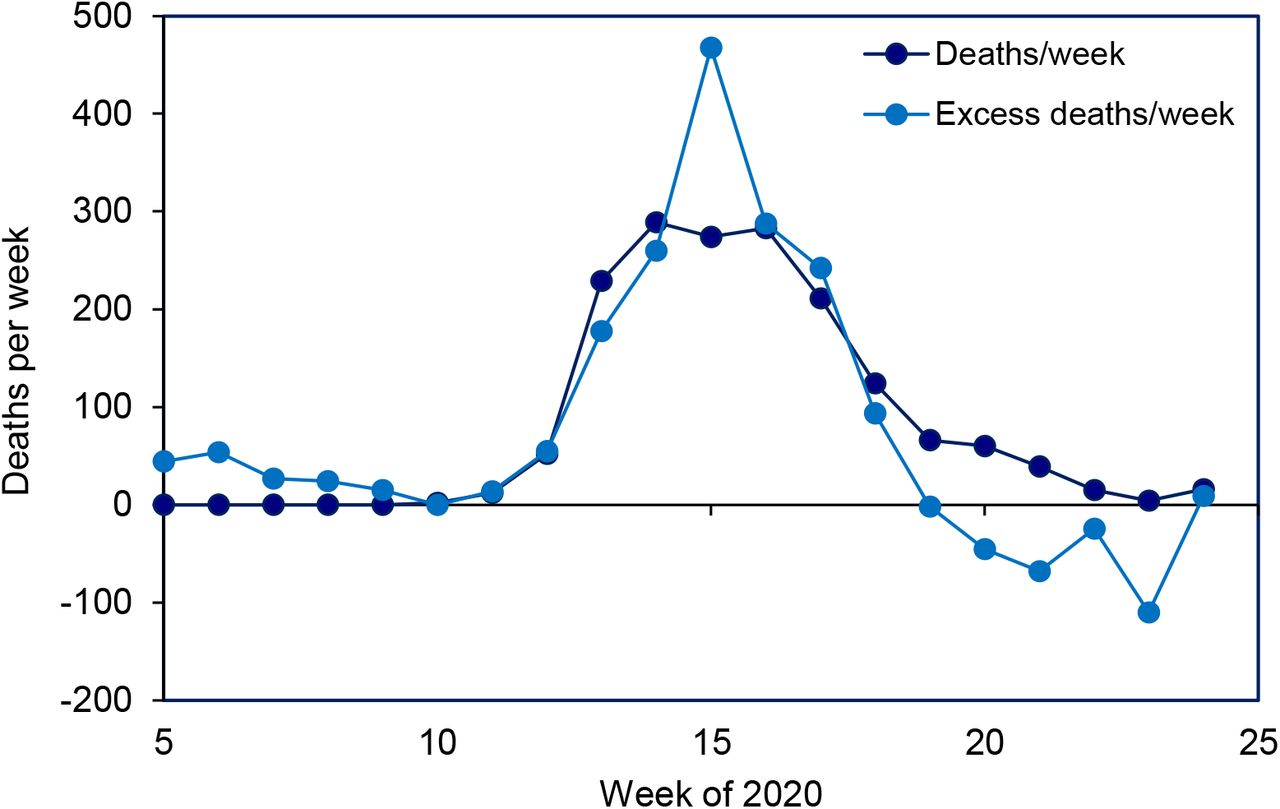
For illustration, Figure 1 shows, with the aid of a dynamic SEIR epidemiological model (Supplementary Materials), how the COVID-19 epidemic in Switzerland might have been contained by flattening the curve. With an estimated basic case reproduction number of R0 = 2.33, the number of deaths reached a maximum of approximately 420 in week 15 (week beginning 6 April), and a total of 1800 deaths had occurred by week 25. If the basic case reproduction number had been higher at the outset (R0 = 3.50 in Figure 1) the epidemic would have been larger (2020 deaths) and narrower, peaking sooner and lasting for a shorter period of time. A lower basic case reproduction number (R0 = 1.75) would have reduced the size of the epidemic, and the 1300 deaths would have occurred over a longer time period (flatter epidemic curve). These calculations are consistent with epidemic theory, which shows how the final size of an epidemic (proportion of people infected, p) is a monotonically increasing function of R0, through the relationship p = 1 − exp (−pR0) (5).

COVID-19 transmission model (lines) for Switzerland used to illustrate the effect of control methods that reduce the contact rate, for example by physical distancing, so as to flatten the epidemic curve, here described by the number of deaths per week (points). As the basic case reproduction number falls in the epidemic model from R0 = 3.5 to 2.33 to 1.75, the maximum number of deaths per week is reduced and delayed, and the epidemic becomes smaller in size, causing fewer deaths in total. Data are the reported numbers of COVID-19 deaths (dark blue points) and all excess deaths in Switzerland (scaled to illustrate and confirm the time trend, light blue points). The transmission model and data (13). are described further in the Supplementary Materials.
Does this theory explain the differences in COVID-19 epidemics across European countries? Did countries with more effective COVID-19 control programmes – those that reported fewer cases and deaths – have flatter epidemic curves? How has the scale and shape of European epidemics been changed by interventions, especially physical distancing under lockdown?
Figure 2 approaches these questions with respect to the number and distribution of deaths through time for 24 European countries. Rather than using a dynamic epidemiological model to describe these epidemics, such as an SEIR model which is constrained by assumptions of, for example homogeneous mixing and exponentially distributed time periods (Supplementary Materials), we used an empirical model (skew-logistic) to measure the rate of epidemic growth, the maximum number of deaths per week, the period of growth (time from one death to the maximum number of weekly deaths), and the rate of decline. The empirical model gives an excellent description of COVID-19 epidemics across Europe; it is also more discriminating between epidemics than estimates of the time-varying case reproduction number (Supplementary Materials, Figure S6).
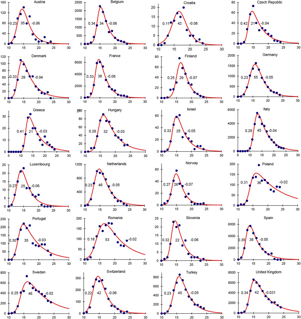
Epidemic curves for 24 European countries based on the number of deaths (points, vertical axis) reported each week (horizontal axis), described by an empirical model (red line) which is used to calculate the epidemic growth rate, the duration of epidemic growth and the rate of decline in each country (inset figures, left to right). Although the data are reported daily, and growth rates and durations are given in days, the model is fitted to the weekly numbers of deaths in order to sum over the 7-day reporting cycle (Supplementary Materials). Data source (13).
The total number of deaths reported by each of the 24 countries up to 20 June varied more than 100-fold, from approximately 100 in Croatia to 42,000 in the United Kingdom. The average growth rate of epidemics was 0.28/day (95%CI 0.006/day), average doubling time 2.7 days), the average duration of epidemic growth was 36 days (95%CI 4.0 days), and the average rate of decline was −0.05/day (95%CI ± 0.001/day, average halving time 17.2 days).
The total number of reported deaths was 5.6 (95%CI 0.29) times the peak number of weekly deaths across the 24 countries (R2 = 0.98, Figure 3a). The principal determinant of variation in the number of deaths among countries was neither the rate of epidemic growth (R2 = 0.01, Figure 3b) nor the rate of decline (R2 = 0.03, Figure 3c), but rather the duration of growth – the period over which the epidemic was allowed to expand (t = 3.91, p < 0.001, R2 = 0.41, Figure 3d).
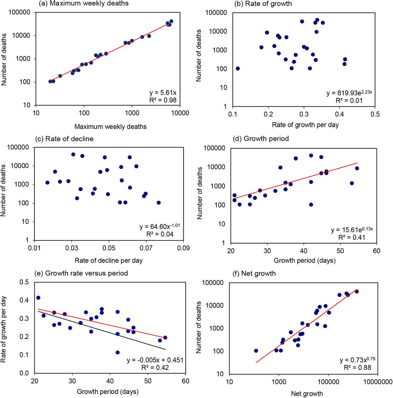
Determinants of the number of COVID-19 deaths in 24 European countries. (a) Relation between the maximum weekly number of deaths and the total number of reported deaths, shown on logarithmic scales. (b)-(d) Numbers of deaths in relation to (b) the rate of epidemic growth per day, (c) the rate of epidemic decline per day and (d) the period or duration of epidemic growth (days), (e) Growth rate and period are inversely related (red line); to reduce epidemic size, growth rate would need to fall more quickly (black line, equivalence) to offset longer periods of growth. (f) Net growth G = egd is closely associated with the total number of reported deaths. Each panel gives the regression equation (red line) along with the fraction of the variation explained by each independent variable (R2). (f) Data source (13).
Longer periods of epidemic growth were associated with lower growth rates (R2 = 0.37, Figure 3e), the expected consequence of physical distancing (Figure 1). Against expectation, however, slower growth rates were associated with more deaths rather than fewer deaths overall. The reason is that, in comparisons between countries, slower growth was more than offset by longer periods of growth (the red line lies above the black line of equivalence in Figure 1e).
The product of the rate (g) and duration of growth (d) defines net epidemic growth – how much an outbreak expands in size during the growth period. Net growth, measured by G = egd, accounted for 88% of the inter-country variation in the number deaths (t = 12.4, p < 0.001, R2 = 0.88; Figure 3f). Although such a relationship is expected in principle, it is surprising that theory is upheld so faithfully in data collected in different ways across 24 diverse European countries.
Countries with larger populations generally reported more deaths (t = 6.83, p < 0.001, R2 = 0.68); however, in multiple regression analysis, population size did not explain significantly more of the inter-country variation in deaths (t = 1.75, p > 0.05) than net growth, G (t = 6.39, p < 0.001). In other words, the effect of population size is accommodated within the measure of net growth. There is a hint in these data that the size of a COVID-19 epidemic increased more than linearly with national population size (N, millions), such that the number of deaths, D = 51.1N1.32. The implication is that population size is more than an epidemic scaling factor, with effects that are not fully captured as deaths per capita. However, the exponent 1.32 is not significantly greater than unity (t = 1.64, p > 0.05). In any event, epidemics expanded more, and caused more deaths, in countries with larger populations.
Because the duration of growth (Figure 3d) and net growth (Figure 3f) can account for much of the inter-country variation in numbers of deaths, we expect, in the data as well as in theory, the timing of interventions to be a determinant of epidemic size. One summary measure of the implementation of control measures is the Government Response Stringency Index, a composite metric of lockdown policies based on nine indicators including school closures, workplace closures, and travel bans, with a score for each country varying between 0 and 100% (6). Figure 4 shows how the total number of deaths (D) reported from each country up to 20 June increased in relation to the cumulative number that had been reported when the Stringency Index reached or exceeded 70% (DL). The form of the power relationship is D ≈ 200DL0.8. The geometric mean ratio of D to DL is 128 in both model and data, but with greater variation in the data (95%CI 155) than in the fitted model (95%CI 19). Based on the model relationship, the expected number of deaths varied from 60 to 200 times the number at lockdown, as the latter ranged from its highest (more than 300 in Sweden) to lowest values (zero in e.g. Croatia, Romania, Slovenia).
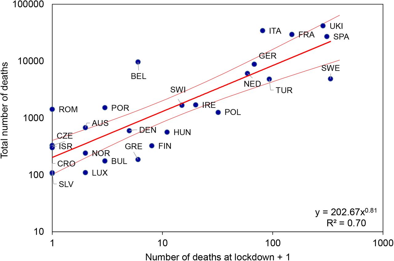
Total numbers of COVID-19 deaths (D) reported from 26 European countries (the 24 in Figures 2 and 3 plus Bulgaria and Slovenia) in relation to the number of deaths (plus 1, to avoid zero on a logarithmic scale) that were reported at the time of lockdown (DL), i.e. the date on which a country achieved a Stringency Index of 70% or more. The form of the power relationship (red line) is D = 200DL0.81, and the geometric mean ratio D/DL in model and data is 128. Errors on the regression line are 95%CI. Further information and analysis, including full country names, are in the Supplementary Materials. Data sources (6, 13).
To illustrate the differences between countries, Luxembourg achieved a Stringency score of 72% on 16 March having recorded only 1 death; by 20 June they had recorded 110 deaths. Spain achieved the same Stringency score of 72% a day later on 17 March, having recorded 309 deaths; by 20 June, Spain had recorded 27,000 deaths.
The outlying countries in Figure 4 raise questions for further investigation: Belgium locked down (73% Stringency) on 18 March with 5 deaths, and yet the epidemic grew faster than average (0.34/day) and for longer than average (34 days), generating a relatively high number of deaths. Unusually, Belgium has reported more COVID-19 deaths than all excess deaths, but only around 15% more (Supplementary Materials), whereas observed and expected COVID-19 deaths differ by a factor of 10 in Figure 4. Sweden never achieved a Stringency score as high as 70% (maximum 46%) and reported a relatively large number of deaths (4900) among Scandinavian countries (fewer than 600 in each of Denmark and Norway). However, the general relationship in Figure 4 predicts a far higher death toll. The reasons why Belgium and Sweden do not conform to the general pattern in Figure 4 remain to be determined.
In conclusion, this analysis shows that European countries reporting fewer COVID-19 deaths had flatter epidemic curves (Figure 2), but not in the way anticipated by simple epidemic theory (Figure 1). Countries with fewer deaths overall did have smaller peak death rates, as expected, but they suffered fewer COVID-19 deaths due to shorter rather than longer periods of epidemic growth. In these comparisons between countries, longer epidemics were generally larger epidemics.
The cross-country comparison in Figure 4 shows that the overall death toll was lower in countries that locked down earlier, when fewer deaths had been reported. But the inference that a country with high COVID-19 mortality could have been like a country with a low mortality, had it acted sooner, comes with a caution: controlling COVID-19 epidemics through early intervention appears to be harder in countries with larger populations, for reasons that are not explained by this study.
Notice, in addition, that epidemic expansion was greater in more populous countries, not because they imported more infections (a scaling factor), though that might also be true (7, 8), but rather because they had epidemics that grew for longer (a multiplication factor).
Taken together, these data expose the perils of delayed action during an epidemic with an average doubling time as short as 3 days. At this rate of growth, the daily death toll would have increased by a factor of ten within 9 days, which is shorter than the average time delay from one death to the time of lockdown, 11 days (ranging from −6 days in the Czech Republic to +43 days in Sweden). In effect, a COVID-19 epidemic in the average European country would have expanded more than ten-fold within the time it took to impose lockdown.
The need for speed is expected to apply to resurgent epidemics too. Behind this analysis lies the supposition, supported by antibody surveys (9–11), that only a small fraction of Europe’s population as been exposed to infection (of the order of 5–10%), albeit a fraction that varies among countries. Like others (1, 3, 12), we assume that new COVID-19 outbreaks will threaten large numbers of susceptible people across Europe, a view reinforced by renewed outbreaks in several countries during June 2020. Facing the risk of further outbreaks of COVID-19, this analysis points to the benefits of taking action without delay.
Data Availability
All data are publicly available.
Supplementary Materials
Materials and methods
This supplement to the main text provides data sources, methods of data analysis, the mathematical model of COVID-19 dynamics and additional data and Figs.
Data sources
This analysis is based on COVID-19 deaths reported from 26 European countries, for which the abbreviations are tabulated below (1). We used reported deaths because they are likely to be more accurate than reported cases, both in absolute magnitude (scale of the epidemic) and in the distribution of deaths through time (shape of the epidemic). However, a comparison of COVID-19 deaths and all excess deaths in Switzerland (Fig 1, Fig S3 below) questions the completeness of death reports at the peak of the epidemic. Nevertheless, the large differences in numbers of reported deaths between countries, and in number of deaths per capita, are very unlikely to be due solely to differences in diagnostic and reporting methods (2). Indeed, the clear patterns of association in Figs 3 and 4 of the main text suggest that both the data and the empirical model portray real effects, rather than artefacts, of COVID-19 epidemics across the 26 countries studied in this investigation.
SEIR model of COVID-19 transmission dynamics
Fig 1 was constructed with a compartmental model of SARS CoV-2 transmission, framed in ordinary differential equations, and representing a homogeneously mixing population divided among susceptible, exposed, infectious and recovered or died (SEIR), as follows:

The SEIR model. The compartments denote those in the population that are Susceptible, Exposed, Infected and Recovered.
The variables S, E, I and R satisfy the ordinary differential equations:


A convenient recent reference is Ma (3), though we have adjusted the notation here, reserving certain symbols for use in other standard ways.
As this discussion focuses on the number that die due to the epidemic we adjust the SEIR model by splitting R, those that recover, to distinguish between Z, those that die, from those that recover well. This arrangement is depicted in Fig S2, and is a simplified version of that used by Dagpunar (4), which discusses the outcomes of hospitalization.

Adjustment of the SEIR model where R is divided into two compartments, R \ Z, those that recover and Z, those that die; where pR is the proportion that recover.
We allow this adjusted SEIR model to depend on certain parameters with the understanding that once these parameters are known the behaviour of the SEIR model is completely specified. There are nine parameters in the model:
The last parameter τ is used to modify the last differential equation (4) to:

We denote by θ = (b1, b2, …, b9), the vector of parameters. With θ given, the four differential equations (1), (2), (3) and (5) can be solved by numerical integration to give the trajectories
 where t is the day and N is the number of days of interest. However, the parameters are assumed unknown. We therefore used the standard method of Maximum Likelihood (ML) as given for example in Cheng (5) to estimate the parameter values.
Here we outline the approach (called fitting the model) used to estimate the parameters from a sample of observed daily deaths, this being used to prepare Fig 1 in the main text. Let the sample of observed number of daily deaths be denoted by
 where zt is the number of deaths on day t and N is the number of days observed. If the observations were made without error and if, with the right parameter values are correct for θ, then the death trajectory {Z(t, θ) t = 1,2, …, N} would match the observed deaths Z in (7). So the model would be clearly successful in explaining deaths.
To include statistical uncertainty in the model we assume instead
 where e(t) is random error. For simplicity the e(t) are assumed to be normally and independently distributed (NID) with standard deviation σ, i.e.

The logarithm of the distribution of the sample is then
 where Z is the random argument, and the parameters θ are fixed. In ML estimation, this is turned on its head so that Z is simply the known sample of observations now regarded as fixed and we write L as L(Z|θ) = L(θ|Z)) calling it the (log)likelihood to indicate that it is now treated as a function of θ. The ML estimator
  is simply the value of θ at which L(θ| Z) is maximized. i.e.

Nelder-Mead numerical search for the maximum was used. This goes through different θi i=1, 2, 3,… comparing the different L(θ i, |z) to find  the best θ.
To simplify description of the estimation process, only fitting to deaths data, Z as in (7) has been described, but the method extends straightforwardly to include other data samples. For example
 where yt is the number of active cases on day t. Fitting simultaneously to both Y and Z can be carried out by adding to the right-hand side of (10) a corresponding set of terms for Y. Numerical solution of the differential equations requires initial values for S, E, I, R. These are essentially scale invariant with (S + E + I + R) constant and independent of t. So the numerical integration can conveniently be done using S(0, θ) = 1, E(0, θ) some small quantity subsequently adjustable as its initial value e0 is a parameter; with I and R also initially zero. The population size, also a parameter, is only needed to provide scaled values S, E, I, R at each step for comparison with the data Y and Z.
Epidemic shape and scale
Flattening the epidemic curve: the model Swiss epidemics in Fig 1 have been scaled for peak case incidence. Reducing R0 from 3.5 to 2.33 to 1.75, through physical distancing (lowering the contact rate), generates epidemics that are distributed over a longer time period, with slower rates of growth and decline. This recalling of Fig 1 is to illustrate that R0 changes the shape as well as the size of epidemics.
Model epidemics for Switzerland in Fig 1 differ in shape as well as size; they are not scale invariant. Fig S3 adjusts the peak sizes of epidemics in Fig 1 to show more clearly the differences in shape, i.e. the different distribution of deaths through time when an epidemic is “flattened” by reducing the case reproduction number.
Comparison of reported COVID-19 deaths and all excess deaths in Switzerland
In Switzerland, the relatively flat peak in reported COVID-19 deaths (Fig 1 of the main text) differs from the estimated number of excess deaths (week 14), suggesting that COVID-19 deaths might have been under-reported in that week (Fig S4).

Reported weekly COVID-19 deaths in Switzerland (filled bars) compared with all excess deaths. Excess deaths are the number in each week of 2020, compared with the average for 2015-19, calculated as the z-score (mean/standard deviation of mortality) multiplied by 40 to permit comparison with COVID-19 deaths (cf Fig 1 of the main text). Data on z-scores are from (6), which does not publish absolute estimates of excess deaths.
The number of excess deaths reported from European countries was approximately 29% greater than the number of COVID-19 deaths (in 8 countries for which estimates have been published; Fig S5) (7). This is a small difference within each country, in comparison with the 100-fold difference COVID-19 deaths reported between countries.

Empirical model of epidemic growth and decline
Although the SEIR model is based on epidemiological principles, it does not accurately describe all of the European COVID-19 epidemics. In particular, the SEIR model does not easily replicate the slow rates of epidemic decline. For this reason we used a skew-logistic model to describe European epidemics:
 where f(t) is the number of deaths per unit time. The growth rate of the epidemic is b, and f(t) converges to zero at a rate of decline d = b − 2c when t → ∞. Parameter τ positions the epidemic along the time axis. The model can be fitted to data – here deaths in each time interval – either by least squares (LSQ) or maximum likelihood methods (MLE). We fitted the model to data from 24 countries for which there were sufficient reported deaths (Figs 2 and 3 of the main paper), but added Bulgaria and Slovenia for the analysis in Fig 4. Examples of the estimates shown in Fig 2, with 95% CI from MLE are:
An alternative way to characterize epidemics, conceptually consonant with the SEIR model, is by means of the time varying case reproduction number, Re. Estimates of Re shown in Fig S5 are based on reported deaths and calculated by methods described in Cori et al (8), implemented by ETH Zurich (9). Re for each day is presented as the continuously varying (retrospective) average. While commonly used and reported, Re does not characterize and distinguish European epidemics as effectively as the empirical model (Fig S6).
Time trends in Re are similar for Germany and the United Kingdom (Fig S5b), although they do show the lower rate of epidemic decline in the UK. In general, however, the skew-logistic model provides a more useful set of parameters to separate these two countries (and others), as in the shaded entries to the Table below. Besides the rate of decline, the two countries experienced differences in epidemic growth rate, the duration of epidemic growth, net growth, and the number of deaths at the epidemic peak, as shown in the following Table:

Estimates of the time varying reproduction number, Re, for (a) 10 European countries and (b) Germany and the United Kingdom, with overlapping lower and upper estimates of the median. Source (9).


