
Abstract
Understanding the outbreak dynamics of the COVID-19 pandemic has important implications for successful containment and mitigation strategies. Recent studies suggest that the population prevalence of SARS-CoV-2 antibodies, a proxy for the number of asymptomatic cases, could be an order of magnitude larger than expected from the number of reported symptomatic cases. Knowing the precise prevalence and contagiousness of asymptomatic transmission is critical to estimate the overall dimension and pandemic potential of COVID-19. However, at this stage, the effect of the asymptomatic population, its size, and its outbreak dynamics remain largely unknown. Here we use reported symptomatic case data in conjunction with antibody seroprevalence studies, a mathematical epidemiology model, and a Bayesian framework to infer the epidemiological characteristics of COVID-19. Our model computes, in real time, the time-varying contact rate of the outbreak, and projects the temporal evolution and credible intervals of the effective reproduction number and the symptomatic, asymptomatic, and recovered populations. Our study quantifies the sensitivity of the outbreak dynamics of COVID-19 to three parameters: the effective reproduction number, the ratio between the symptomatic and asymptomatic populations, and the infectious periods of both groups. For nine distinct locations, our model estimates the fraction of the population that has been infected and recovered by Jun 15, 2020 to 24.15% (95% CI: 20.48%-28.14%) for Heinsberg (NRW, Germany), 2.40% (95% CI: 2.09%-2.76%) for Ada County (ID, USA), 46.19% (95% CI: 45.81%-46.60%) for New York City (NY, USA), 11.26% (95% CI: 7.21%-16.03%) for Santa Clara County (CA, USA), 3.09% (95% CI: 2.27%-4.03%) for Denmark, 12.35% (95% CI: 10.03%-15.18%) for Geneva Canton (Switzerland), 5.24% (95% CI: 4.84%-5.70%) for the Netherlands, 1.53% (95% CI: 0.76%-2.62%) for Rio Grande do Sul (Brazil), and 5.32% (95% CI: 4.77%-5.93%) for Belgium. Our method traces the initial out- break date in Santa Clara County back to January 20, 2020 (95% CI: December 29, 2019 - February 13, 2020). Our results could significantly change our understanding and management of the COVID-19 pandemic: A large asymptomatic population will make isolation, containment, and tracing of individual cases challenging. Instead, managing community transmission through increasing population awareness, promoting physical distancing, and encouraging behavioral changes could become more relevant.
1. Motivation
Since its outbreak in December 2019, the COVID-19 pandemic has rapidly swept across the globe and is now affecting 188 countries with more than 5 million cases reported worldwide [9]. In the early stages of a pandemic, doctors, researchers, and political decision makers mainly focus on symptomatic individuals that come for testing and address those who require the most urgent medical attention [14]. In the more advanced stages, the interest shifts towards mildly symptomatic and asymptomatic individuals who–by definition–are difficult to trace and likely to retain normal social and travel patterns [34]. In this manuscript, we collectively use the term “asymptomatic” for individuals who have mild symptoms that are not directly associated with COVID-19 or display no symptoms at all. Recent antibody seroprevalence studies suggests that the number of asymptomatic COVID-19 cases outnumbers the symptomatic cases by an order of magnitude or more [3, 4, 8, 11, 13, 17, 23, 28, 30, 37, 46, 47, 52, 53, 56, 54, 55, 59, 60, 62, 64, 66, 68]. Estimating the prevalence and contagiousness of these asymptomatic cases is critical since it will change our understanding of the overall dimension and the pandemic potential of COVID-19 [15]. Yet, at this stage, the effect of the asymptomatic population, its size, and its outbreak dynamics remain largely unknown.
The first evidence of asymptomatic individuals in a family cluster of three was reported in late January, where one individual was mildly symptomatic and two remained asymptomatic, with normal lymphocyte counts and chest computer tomography images, but positive quantitative reverse transcription polymerase chain reaction tests [41]. As of today, more than 50 studies have reported an asymptomatic population, twenty-three of them with a sample size of at least 500 [27], with a median undercount of 20 across all studies, suggesting that only one in twenty COVID-19 cases is noticed and reported. These studies are based on polymerase chain reaction or antibody seroprevalence tests in different subgroups of the population, at different locations, at different points in time [3, 6, 59]. To no surprise, the reported undercount varies hugely, ranging from 3.5 and 5.0 in Luxembourg [56] and Germany [59] to 543 and 627 in Iran [53] and Japan [8] respectively. Most of these studies are currently only available on preprint servers, but an increasing number is now passing peer review, including a study of 1402 individuals in Wuhan City with an undercount of 22.1 [68], a study of 400 health care workers in London with an undercount of 35.0 [65], a community spreading study of 131 patients with influenza-like symptoms in Los Angeles with an undercount of 100.0 [58], and a seroprevalence study in Los Angeles county with an undercount of 43.5 [57]. The reported trend across all studies is strikingly consistent: A much larger number of individuals displays antibody prevalence than we would expect from the reported symptomatic case numbers. Knowing the exact dimension of the asymptomatic population is critical for two reasons: first, to truly estimate the severity of the outbreak, e.g., hospitalization or mortality rates [15], and second, to reliably predict the success of surveillance and control strategies, e.g., contact tracing or vaccination [18].
While there is a pressing need to better understand the prevalence of asymptomatic transmission, it is also be- coming increasingly clear that it will likely take a long time until we can, with full confidence, deliver reliable measurements of this asymptomatic group. In the meantime, mathematical modeling can provide valuable insight into the tentative outbreak dynamics and outbreak control of COVID-19 for varying asymptomatic scenarios [34]. Many classical epidemiology models base their predictions on compartment models in which individuals pass through different stages as they experience the disease [29]. A popular model to simulate the outbreak dynamics of COVID-19 is the SEIR model [14], which is made up of four compartments for the susceptible, exposed, infectious, and recovered populations [2]. Here, to explicitly account for the asymptomatic population, we introduce an SEIIR model, which further divides the infectious population into symptomatic and asymptomatic groups. Similar models have recently been used to study the general role of asymptomatic carriers in disease transmission [42] and to illustrate how asymptomatic individuals have facilitated the rapid spread of COVID-19 throughout China [34], South Korea [63], and Italy [19]. While it is tempting–and easily possible–to introduce many more sub-populations into the model, for example a pre-symptomatic, hospitalized, or mortality group [45], here, we focus on the simplest possible model that allows us to explore the role of the asymptomatic population throughout the COVID-19 pandemic. To systematically probe different scenarios, we combine this deterministic SEIIR model with a dynamic effective reproduction number and adopt machine learning and uncertainty quantification techniques to learn the reproduction number, in real time, and quantify uncertainties in the symptomatic-to-asymptomatic ratio, and the initial exposed and infectious populations [36]. We show that this not only allows us to visualize the dynamics and uncertainties of the dynamic contact rate, the effective reproduction number, and the symptomatic, asymptomatic, and recovered populations, but also to estimate the initial date of the outbreak.
2. Methods
2.1 Epidemiology modeling
We model the epidemiology of COVID-19 using an SEIIR model with five compartments, the susceptible, ex- posed, symptomatic infectious, asymptomatic infectious, and recovered populations. Figure 1 illustrates our SEIIR model, which is governed by a set of five ordinary differential equations,
The SEIIR model contains five compartments for the susceptible, exposed, symptomatic infectious, asymptomatic infectious, and recovered populations. The transition rates between the compartments, β, α, and γ are inverses of the contact period B = 1/β, the latent period A = 1/α, and the infectious period C = 1/γ. The symptomatic and asymptomatic groups have the same latent period A, but they can have individual contact periods Bs = 1/βs and Ba = 1/βa and individual infectious periods Cs = 1/γs and Ca = 1/γa. The fractions of the symptomatic and asymptomatic subgroups of the infectious population are vs and va. We assume that the infection either goes through the symptomatic or the asymptomatic path, but not both for one individual.
 where the fractions of all five populations add up to one, S + E + Is + Ia + R = 1. We assume that both the symptomatic group Is and the asymptomatic group Ia can generate new infections. We introduce these two groups by fractions vs and va of the subjects transferring from the exposed group E. We postulate that the two infectious groups Is and Ia have the same latent period A = 1/α, but can have individual contact periods Bs = 1/βs and Ba = 1/βa to mimic their different community spreading, and individual infectious periods Cs = 1/γs and Ca = 1/γa to mimic their different likelihood of isolation. From the infectious fractions, we can derive the overall contact and infectious rates β and γ from their individual symptomatic and asymptomatic counterparts, βs, βa, γs, and γa,

Similarly, we can express the overall contact and infectious periods B and C in terms of their symptomatic and asymptomatic counterparts, Bs, Ba, Cs, and Ca,

Naturally, the different dynamics for the symptomatic and asymptomatic groups also affect the basic reproduction number R0, the number of new infections caused by a single one individual in an otherwise uninfected, susceptible population,

For a large asymptomatic group va → 1, the basic reproduction number approaches the ratio between the infectious and contact periods of the asymptomatic population, R0 → Ca/Ba, which could be significantly larger than the basic reproduction number for the symptomatic group, R0 = Cs/Bs, that we generally see reported in the literature. To characterize the effect of changes in social behavior and other interventions that may affect contact, we assume that the contact rate β(t) can vary as a function of time [36], but is the same for the symptomatic and asymptomatic groups,

This introduces a time-varying effective reproduction number R(t), which is an important real time characteristic of the current outbreak dynamics. For the special case when the dynamics of the symptomatic and asymptomatic groups are similar, i.e., βs = βa = β and γs = γa = γ, we can translate the SEIIR model (1) into the classical SEIR model (6) with four compartments, the susceptible, exposed, infectious, and recovered populations [35]. For this special case, we can back-calculate the symptomatic and asymptomatic groups from equation (6.3) as Is = vs I and Ia = va I. Figure 2 illustrates the SEIR model, which is governed by a set of four ordinary differential equations [25],
The SEIR model contains four compartments for the susceptible, exposed, infectious, and recovered populations. The transition rates between the compartments, β, α, and γ are inverses of the contact period B = 1/β, the latent period A = 1/α, and the infectious period C = 1/γ. If the transition rates are similar for the symptomatic and asymptomatic groups, the SEIIR model simplifies to the SEIR model with Is = vsI and Ia = vaI.
2.3 Seroprevalence studies
We consider seroprevalence studies where the representation ratio, the ratio between the amount of seropreva- lence samples and the representative population, is larger than 0.02%. Subsequently, we draw the daily number of confirmed reported cases for Heinsberg, Ada County, New York City, Santa Clara County, Denmark, Geneva Canton, Netherlands, Rio Grande do Sul, and Belgium from online data repositories [5, 10, 24, 39, 40, 61]. The symptomatic fraction vs follows from the ratio between the reported confirmed cases for the studied region and the amount of seroprevalence-estimated cases on the last day of the seroprevalence study. Table 1 summarizes the study date, number of samples, representation ratio, population, and symptomatic fraction of each location.
Seroprevalence studies with a representative population larger than 0.02%, location, study date, number of samples, representation ratio, population, and symptomatic fraction vs.
2.3 Uncertainty quantification
Our SEIIR model uses the following set of parameters, ϑ = {A, Cs, Ca, vs, β(t), E0, Is0, Ia0, σ}. To reduce the set of unknowns, we fix the latency period A = 2.5 days and the symptomatic infectious period Cs = 6.5 days [32, 33, 50]. Since the asymptomatic infectious period Ca is unreported, we study three cases with Ca : Cs = 0.5, 1.0, and 2.0, resulting in infectious periods of Ca = 3.25, 6.5, and 13.0 days. We impose the symptomatic fraction of the infectious group, vs to follow the distributions from Table 1. We estimate the remaining parameters including the time- varying contact rate β(t), the initial exposed population E0, and the initial symptomatic and asymptomatic infectious populations Is0 and Ia0 using Bayesian inference. For the time-varying contact rate β(t), we set a log-Gaussian random walk prior, which we construct with weakly informative priors with a drift µRW and a daily step width σRW. For the initial symptomatic infectious population Is0, we set a weakly informative log-normal prior distribution with a mean equal to the amount of detected confirmed cases on day 0 and a standard deviation equal to one. We express the initial asymptomatic infectious population as Ia0 = [1 − vs]/vs Is0, and approximate the initial exposed population as E0 = [A/Cs] [Is0 + Ia0] [12]. Table 2 summarizes the choice of our priors.
Prior distributions for SEIIR model parameters.
For each parameter set, we deterministically calculate the time series of each compartment using an explicit time integrator. For each point in time, we calculate the detected cases, D(t) = Is(t) + Rs(t) with  . By scaling the confirmed reported cases with the total population N, we obtain the relative detected population
  . The day on which each location went into lockdown marks day 0 and the beginning of our simulation. From this day on, we calculate the simulated detected population, D(t) = Is(t) + Rs(t) with
  . We quantify the likelihood of the parameter set and model outcome D(t) in correlation to the reported cases
  , using Student’s t-distribution,

We choose this distribution because it resembles a Gaussian distribution and makes the Markov-Chain Monte Carlo more robust with respect to outliers [7, 31]. Here, σ represents the width of the likelihood  between the time- varying reported and the modeled symptomatic populations. Using Bayes’ rule, we compute the posterior distribution of the parameters [44, 48] to account for the prior knowledge on the parameters and the reported confirmed cases themselves,

Since we cannot describe the posterior distribution over the model parameters ϑ analytically, we adopt approximate- inference techniques to calibrate our model on the available data. We use the NO-U-Turn sampler (NUTS) [26], which is a type of Hamiltonian Monte Carlo algorithm as implemented in PyMC3 [49]. We use four chains, and the first 4 times 500 samples serve to tune the sampler and are later discarded. We use the subsequent 4 times 1000 samples as the posterior distribution for the parameters ϑ. From the converged posterior distribution, we sample multiple combinations of parameters that describe the time evolution of reported cases. Using these posterior samples, we quantify the uncertainty of each parameter based on the reported case data. As such, each parameter set provides a set of values for the initial exposed population E0, the initial symptomatic and asymptomatic populations Is0 and Ia0, the symptomatic fraction vs, and the time evolution of the contact rate β(t). From these values, we quantify the effective reproductive number R(t) and the time evolution of the susceptible, exposed, symptomatic infectious, asymptomatic infectious and recovered populations, S (t), E(t), Is(t), Ia(t), and R(t) and report their values with the associated 95% credible interval.
2.4 Hierarchical asymptomatic infectious period Caestimation
To estimate the asymptomatic infectious period Ca, we combine the confirmed case data from all locations and set up a hierarchical model for Ca. Here we postulate that each location-specific  is drawn from a hyperdistribution Ca. We assume that the initial reproduction number, which is disease-specific, is the same for all locations [16] and is constant during a two-week time window around each local lockdown date: 10 days prior till 3 days (∼ A, the latent period) after each local lockdown date. The priors for these distributions are summarized in Table 3. We perform Bayesian inference as explained above and subsequently use the hierarchical posterior Ca distribution to quantify the time-varying asymptomatic infectious population size at each of the locations after the lockdowns.
Prior distributions for SEIIR-based hierarchical Ca estimation.
2.5. Estimating the outbreak date
For each sample from the posterior distribution, we use the estimated initial exposed population E0 and the estimated initial asymptomatic infectious population Ia0 to estimate the date of the very first COVID-19 case in Santa Clara County [51]. Specifically, for each parameter set, we create an SEIIR model and assume that the outbreak begins with one single asymptomatic infectious individual. We fix the latency and symptomatic infectious periods to A = 2.5 days and Cs = 6.5 days and impose the hierarchically estimated infectious period Ca. For each posterior sample for the exposed, symptomatic infectious, and asymptomatic infectious population size on the lockdown date (March 16, 2020), we use the Nelder-Mead optimization method [20] to find the most probable outbreak origin date. Specifically, we solve the SEIIR model forward in time using an explicit time integration, starting from various start dates before March 16, 2020, and iteratively minimize the difference between the computed exposed, symptomatic, and asymptomatic infectious populations and the sample’s actual exposed, symptomatic, and asymptomatic infectious populations. We concomitantly fit a static contact rate parameter β which is bounded between zero and the posterior sample’s estimated contact rate on day 0, β(0). Repeating this process for each sample of the Bayesian inference generates a distribution of possible origin dates. From this distribution, we compute the most probable origin date and its uncertainty.
3. Results
3.1. Outbreak dynamics of COVID-19 in Santa Clara County
Figure 3 illustrates the outbreak dynamics of COVID-19 in Santa Clara County. To explore the effects of Ca = on the initial effective reproductive number, we started the simulations 10 days before the local lockdown date: March 6, 2020. The black dots highlight the reported cases  from this day forward. Based on these data points, we learn the posterior distributions of our SEIIR model parameters for fixed latent and symptomatic infectious periods A = 2.5 days and Cs = 6.5 days, and for three asymptomatic infectious periods, Ca = 3.25, 6.5, and 13.0 days, from left to right. The gray and green-purple regions highlights the 95% credible intervals on the confirmed cases D(t), top row, and the contact rate β(t), bottom row, based on the reported cases
  , while taking into account uncertainties on the fraction of the symptomatic infectious fraction vs, and the initial exposed and infectious populations E0, Is0, and Ia0. The red, orange, and green histograms on the middle row display the inferred initial exposed and infectious populations, E0, Is0, and Ia0, for the three different asymptomatic infectious periods. The graphs confirm that our dynamic SEIIR epidemiology model is capable of correctly capturing the gradual flattening and deflattening of the curve of confirmed cases in agreement with the decrease in new cases reported in Santa Clara County, top row. The consistent downward trend of the contact rate β(t) after the lockdown date (March 16, 2020) quantifies the efficiency of public health interventions. The different magnitudes in the contact rate highlight the effect of the three different asymptomatic infectious periods Ca: For larger asymptomatic infectious periods Ca, from left to right, to explain the same number of confirmed cases D(t) = Is(t) + Rs(t), the contact rate β(t) has to decrease. On March 6, 2020, the mean contact rate β(t) was 0.688 (95% CI: 0.612 - 0.764) for an infectious period of Ca=3.25 days, 0.529 (95% CI: 0.464 - 0.593) for Ca= 6.5 days, and 0.463 (95% CI: 0.403 - 0.523) for Ca=13.0 days. By March 16, 2020, the day Santa Clara County announced the first county-wide shelter-in-place order in the entire United States, these contact rates β(t) were 0.491 (95% CI: 0.462 - 0.523) for an infectious period of Ca=3.25 days, 0.328 (95% CI: 0.305 - 0.352) for Ca= 6.5 days, and 0.252 (95% CI: 0.234 - 0.271) for Ca=13.0 days.

The simulation learns the time-varying contact rate β(t) for fixed latent and symptomatic infectious periods A = 2.5 days and Cs = 6.5 days, and for three asymptomatic infectious periods Ca = 3.25 days, 6.5 days, and 13.0 days (from left to right). Computed and reported confirmed cases in Santa Clara County, D(t) = Is(t) + Rs(t) and  (top), initial exposed and infectious populations, E0, Is0, and Ia0 (middle), and dynamic contact rate, β(t) (bottom). The gray and green-blue regions highlight the 95% credible intervals on the confirmed cases D(t) (top) and the contact rate β(t) (bottom) based on the reported cases
  , while taking into account uncertainties on the fraction of the symptomatic infectious population vs = Is/I, and the initial exposed and infectious populations E0, Is0, and Ia0.
3.2. Effect of asymptomatic transmission of COVID-19 in Santa Clara County
Figure 4 visualizes the effect of asymptomatic transmission in Santa Clara County. The simulation learns the time-varying contact rate β(t), and with it the time-varying effective reproduction number R(t), top row, for three asymptomatic infectious periods Ca = 3.25 days, 6.5 days, and 13.0 days, from left to right. The effective reproduction number R(t) follows a similar downward trend as the contact rate β(t). For larger asymptomatic infectious periods Ca, from left to right, since R(t) = Cs β(t)/[vs + va Cs/Ca], as Ca increases, Cs/Ca decreases, and R(t) increases. Since R(t) represents the number of new infections from a single case, a decrease below R(t) < 1 implies that a single infectious individual infects less than one new individual, which indicates that the outbreak decays. The dashed vertical lines indicate the date R(t) = 1 during which one infectious individual, either symptomatic or asymptomatic, infects on average one other individual. For an asymptomatic infectious period of Ca=3.25 days, it took until March 28 before Santa Clara County managed to get R(t) below 1 for the first time after the outbreak. For Ca=6.5 days, this only occurred by April 1 and for Ca=13.0 days, this occurred on April 8, 2020. This confirms our intuition that, the larger the asymptomatic infectious period Ca, for example because asymptomatic individuals will not isolate as strictly as symptomatic individuals, the higher the effective reproduction number R(t), and the more difficult it will be to control R(t) by public health interventions. For each of the three cases, the symptomatic infectious, asymptomatic infectious, and recovered population, are shown in the bottom row. For larger asymptomatic infectious periods Ca, from left to right, the total infectious population I increases and its maximum occurs later in time. Specifically, the maximum infectious population since March 6, 2020 amounts to 0.70% (95% CI: 0.43%-0.97%) on March 28, 2020 for Ca = 3.25 days, 1.23% (95% CI: 0.72%-1.75%) on April 2, 2020 for Ca = 6.5 days, and 2.10% (95% CI: 1.25%- 2.94%) on April 7, 2020 for Ca = 13.0 days. For larger asymptomatic infectious periods Ca, from left to right, the recovered population R decreases. Specifically, on June 15, 2020, the recovered population R amounts to 10.85% (95% CI: 7.06%-16.09%) for an infectious period of Ca =3.25 days, 10.20% (95% CI: 6.07%-14.90%) for Ca =6.5 days, and 9.90% (95% CI: 6.07%-13.93%) for Ca =13.0 days. Similarly, and important when considering different exit strategies, the total infectious population, I = Is + Ia, on June 15, 2020 is estimated to 0.39% (95% CI: 0.24%- 0.58%) for Ca =3.25 days, 0.68% (95% CI: 0.40%-1.01%) for Ca =6.5 days, and 1.25% (95% CI: 0.73%-1.77%) for Ca =13.0 days.

The simulation learns the time-varying contact rate β(t), and with it the time-varying effective reproduction number R(t), for fixed latent and symptomatic infectious periods A = 2.5 days and Cs = 6.5 days, and for three asymptomatic infectious periods Ca = 3.25 days, 6.5 days, and 13.0 days (from left to right). The downward trend of the effective reproduction number R(t) reflects the efficiency of public health interventions (top row). The dashed vertical lines mark the critical time period during which the effective reproductive reproduction number fluctuates around R(t) = 1. The simulation predicts the symptomatic infectious, asymptomatic infectious, and recovered populations Is, Ia, and R (bottom row). The colored regions highlight the 95% credible interval for uncertainties in the number of confirmed cases D, the fraction of the symptomatic infectious population vs = Is/I, the initial exposed population E0 and the initial infectious populations Is0 and Ia0.
3.3. Outbreak dynamics of COVID-19 worldwide
Figure 5 illustrates the hierarchical asymptomatic infectious period Ca estimation for nine locations that reported COVID-19 antibody prevalence in a representative sample of the population: Heinsberg (NRW, Germany), Ada County (ID, USA), New York City (NY, USA), Santa Clara County (CA, USA), Denmark, Geneva Canton (Switzer- land), Netherlands, Rio Grande do Sul (Brazil) and Belgium. This estimate assumes an initial fixed reproduction number R0 = 3.87 (95%CI: 3.01-4.66) during a two-week window before lockdown which results in an asymptomatic infectious period of Ca = 5.76 (95%CI: 3.59-8.09) days. With this value, we simulate the outbreak dynamics of COVID-19 in all nine locations. Figure 6 illustrates the learnt effective reproduction number R(t), and the symp- tomatic and asymptomatic infectious populations Is and Ia, and the recovered population R for all nine locations. Here, we assume fixed latent and infectious periods of A = 2.5 days, Cs = 6.5 days, and the hierarchical asymptomatic infectious period Ca = 5.76 (95%CI: 3.59-8.09) days from Figure 5. For all nine locations, the calculated metrics display the fine balance between the dynamics of the effective reproduction number and the control of the epidemic outbreak. The downward trend of the effective reproductive number R(t) quantifies how fast each location managed to control the spreading of COVID-19. The dashed vertical line indicates the first time each location managed to lower the effective reproduction below R(t) = 1 after lockdown. This critical transition occurred on March 20 for Heinsberg, April 4 for Ada County, April 28 for New York City, March 30 for Santa Clara County, April 8 for Denmark, April 2 for Geneva, April 14 for the Netherlands, June 8 for Rio Grande do Sul and April 11 for Belgium. Based on our simulations, the maximum infectious population size amounted to 3.54% (95% CI: 2.96%-4.11%) on March 19 in Heinsberg, 0.47% (95% CI: 0.41%-0.55%) on May 5 in Ada County, 6.11% (95% CI: 5.99%-6.21%) on April 13 in New York City, 1.11% (95% CI: 0.69%-1.65%) on March 29 in Santa Clara County, 0.38% (95% CI: 0.27%-0.50%) on April 9 in Denmark, 2.10% (95% CI: 1.65%-2.69%) on April 2 in Geneva, 0.63% (95% CI: 0.57%-0.68%) on April 15 in the Netherlands, 0.28% (95% CI: 0.14%-0.48%) on June 8 in Rio Grande do Sul, and 0.70% (95% CI: 0.62%-0.78%) on April 11 in Belgium. On Jun 15, 2020, the estimated recovered population reached 24.15% (95% CI: 20.48%-28.14%) in Heinsberg, NRW, Germany 2.40% (95% CI: 2.09%-2.76%) in Ada County, ID, USA 46.19% (95% CI: 45.81%-46.60%) in New York City, NY, USA 11.26% (95% CI: 7.21%-16.03%) in Santa Clara County, CA, USA 3.09% (95% CI: 2.27%-4.03%) in Denmark 12.35% (95% CI: 10.03%-15.18%) in Geneva Canton, Switzerland 5.24% (95% CI: 4.84%-5.70%) in Netherlands 1.53% (95% CI: 0.76%-2.62%) in Rio Grande do Sul, Brazil 5.32% (95% CI: 4.77%-5.93%) in Belgium.

Assuming an initial fixed reproduction number R0 = 3.87 (95%CI: 3.01-4.66) [16], the simulation generates histograms of the asymptomatic infectious period Ca for each location based on the location-specific symptomatic fraction vs. The black dots and grey regions represent the reported and simulated detected cases  and D(t) respectively. The hierarchical hyperdistribution for the asymptomatic infectious period results in Ca = 5.76 (95%CI: 3.59-8.09) days, right histogram.

Dynamic effective reproduction number R(t) and symptomatic, asymptomatic, and recovered populations at all nine locations. The simulation learns the time-varying contact rate β(t), and with it the time-varying effective repro- duction number R(t), to predict the symptomatic infectious, asymptomatic infectious, and recovered populations Is, Ia, and R, for fixed latent and infectious periods A = 2.5 days, Cs = 6.5 days, the hierarchical asymptomatic infectious period Ca = 5.76 (95%CI: 3.59-8.09) days from Figure 5. The dashed vertical lines mark the the first time each location managed to lower the effective reproduction below R(t) = 1 after lockdown. The colored regions highlight the 95% credible interval for the effective reproductive number R(t) (top), the symptomatic and asymptomatic populations Is and Ia, and the recovered population R (bottom plots), for uncertainties in the number of confirmed cases D, the fraction of the symptomatic infectious population vs, the initial exposed population E0, and the initial infectious populations Is0 and Ia0.
3.4. Estimating the outbreak date
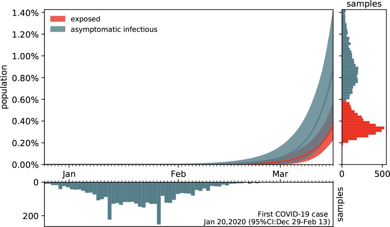
Figure 7 shows the estimated outbreak date of COVID-19 in Santa Clara County. For fixed latent and symptomatic infectious periods A = 2.5 days and Cs = 6.5 days, and for the hierarchically estimated asymptomatic infectious periods Ca = 5.76 (95%CI: 3.59-8.09) days, the graph highlights the estimated date of the first COVID-19 case in the county. Based on the reported case data from March 16, 2020 onward, and taking into account uncertainty on the fraction of the symptomatic infectious population vs, on the initial exposed population E0, and on the initial symptomatic and asymptomatic infectious populations Is0 and Ia0, we systematically backtracked the date of the first undetected infectious individual. Our results suggest that the first case of COVID-19 in Santa Clara County dates back to January 20, 2020 (95% CI: December 29, 2019 - February 13, 2020).
Estimated date of the first COVID-19 case in Santa Clara County for fixed latent and symptomatic infectious periods A = 2.5 days and Cs = 6.5 days, and for the hierarchical asymptomatic infectious period Ca = 5.76 (95%CI: 3.59-8.09) days from Figure 5. The colored regions in the main plot highlight the 95% credible interval for the time evolution of the exposed and asymptomatic infectious populations E and Ia estimated based on the reported cases  from March 16, 2020 onward and taking into account uncertainties on the fraction of the symptomatic infectious population vs = Is/I, and the exposed and asymptomatic infectious populations E0 and Ia0 on March 16, 2020 (right plot). The bottom plot histogram shows the distribution of the most probable origin dates to January 20, 2020 (95% CI: December 29, 2019 - February 13, 2020).
4. Discussion
A key question in understanding the outbreak dynamics of COVID-19 is the dimension of the asymptomatic pop- ulation and its role in disease transmission. Throughout the past three months, dozens of studies have been initiated to quantify the fraction of the general population that displays antibody prevalence but did not report symptoms of COVID-19. Here we assume that this subgroup of the population has been infected with the novel coronavirus, but has remained asymptomatic, or only displayed mild symptoms that were not directly reported in the context of COVID-19. We collectively map this subgroup into an asymptomatic population and additively decompose the total infectious population, I = Is + Ia, into a symptomatic group Is and an asymptomatic group Ia. We parameterize this decomposition in terms of a single scalar valued parameter, the symptomatic fraction vs. Within this paradigm, we can conceptually distinguish two scenarios: the special case for which both subgroups display identical contact rates β, latent periods A, and infectious periods C, and the general case for which these transition dynamics are different.
For comparable dynamics, the size of the asymptomatic population does not affect overall outbreak dy- namics
For the special case in which both subgroups display identical contact rates β, latent rates α, and infectious rates γ [67], our study shows that the overall outbreak dynamics can be represented by the classical SEIR model [25] using equations (6). Importantly, however, since the reported case data only reflect the symptomatic infectious and recovered groups Is and Rs, the true infectious and recovered populations I = Is/vs and R = Rs/vs could be about an order of magnitude larger than the SEIR model predictions. From an individual’s perspective, a smaller symptomatic group vs, or equivalently, a larger asymptomatic group va = [1 − vs], could have a personal effect on the likelihood of being unknowingly exposed to the virus, especially for high-risk populations: A larger asymptomatic fraction va would translate into an increased risk of community transmisson and would complicate outbreak control [15]. From a health care perspective, however, the special case with comparable transition dynamics would not pose a threat to the health care system since the overall outbreak dynamics would remain unchanged, independent of the fraction va of the asymptomatic population: A larger asymptomatic fraction would simply imply that a larger fraction of the population has already been exposed to the virus–without experiencing significant symptoms–and that the true hospitalization and mortality rates would be much lower than the reported rates [27].
For different dynamics, the overall outbreak dynamics depend on both size and infectiousness of the asymptomatic group
For the general case in which the transition rates for the symptomatic and asymptomatic groups are different, the overall outbreak dynamics of COVID-19 become more unpredictable, since little is known about the dynamics of the asymptomatic population [42]. To study the effects of different dynamics between the symptomatic and asymptomatic groups, we decided to collectively represent a lower infectivity of the asymptomatic population through a smaller infectious period Ca < Cs and a lack of early isolation of the asymptomatic population through a larger infectious period Ca > Cs, while, for simplicity, keeping the latent period A and contact rate β similar across both groups [33]. Our study shows that the overall reproduction number, R(t) = [Ca Cs]/[vs Ca + va Cs] β(t), and with it the outbreak dynamics, depend critically on the fractions of the symptomatic and asymptomatic populations vs and va and on the ratio of the two infectious periods Cs and Ca. To illustrate these effects, we report the results for three different scenarios where the asymptomatic group is half as infectious, Ca = 0.5 Cs, equally infectious, Ca = Cs, and twice as infectious Ca = 2.0 Cs as the symptomatic group for Santa Clara County. The second case, the middle column in Figures 3 and 4, corresponds to the special case with comparable dynamics and similar parameters. Our learnt asymptomatic infectious periods of Ca = 5.76 days in Figure 5 suggest that Ca is smaller than the symptomatic infectious period of Cs = 6.5 days and that the asymptomatic population is slightly less infectious as the symptomatic population. This can be a combined effect of less viral shedding as opposed to the symptomatic individuals, whilst concomitantly having more contacts because the asymptomatic individual does not realize he/she is spreading the disease.
Dynamic contact rates are a metric for the efficiency of public health interventions
Classical SEIR epi- demiology models with static parameters are well suited to model outbreak dynamics under unconstrained conditions and predict how the susceptible, exposed, infectious, and recovered populations converge freely toward the endemic equilibrium [25]. However, they cannot capture changes in disease dynamics and fail to converge towards a temporary equilibrium before the entire population has become sufficiently immune to prevent further spreading [45]. To address this limitation, we introduce a time-dependent contact rate β(t), which we learn dynamically from the reported case data. Figures 3 and 6 demonstrate that our approach can successfully identify a dynamic contact rate that not only decreases monotonically, but is also capable of reproducing local contact fluctuations. With this dynamic contact rate, our model can capture the characteristic S-shaped COVID-19 case curve that plateaus before a large fraction of the population has been affected by the disease, resembling a Gompertz function. Previous studies have inferred discrete date points at which the contact rates vary [7] or used sliding windows over the amount of novel reported infections [43] to motivate dynamic contact rates. As such, our framework provides a model-based method for statistical inference of virus transmissibility: It naturally learns the most probable contact rate from the changing time evolution of new confirmed cases and concomitantly quantifies the uncertainty on that estimation.
The dynamics of the asymptomatic population affect the effective reproduction number
Our analysis in equations (4) and (5) and our simulations in Figure 4 illustrate how asymptomatic transmission affects the effective reproduction number, and with it the outbreak dynamics of COVID-19. Our results show that, the larger the infectious period Ca of the asymptomatic group, the larger the initial effective reproduction number, R(t) = Cs β(t)/[vs + va Cs/Ca], and the later the drop of R(t) below the critical value of one. A recent study analyzed the dynamics of the asymptomatic population in three consecutive windows of two weeks during the early outbreak in China [34]. The study found relatively constant latency and infectious periods A and C, similar to our assumption, and a decrease in the contact rate β = 1.12, 0.52, 0.35 days−1 and in the effective reproduction number R(t) = 2.38, 1.34, 0.98, which is consistent with our results. However, rather than assuming constant outbreak parameters within pre-defined time windows, our study learns the effective reproduction number dynamically, in real time, from the available data. Figures 4 and 6 demonstrate that we can successfully learn the critical time window until R(t) drops below 1, which, in Santa Clara County, took till March 28 for Ca =3.25 days, till April 1 for Ca = 6.5 days and till April 8 for Ca = 13.0 days. Our findings are consistent with the observation that the basic reproduction number will be over-estimated if the asymptomatic group has a shorter generation interval, and underestimated if it has a longer generation interval than the symptomatic group [42]. Naturally, these differences are less pronounced under current conditions where the effective reproduction number is low and the entire population has been sheltering in place. It will be interesting to see if the effects of asymptomatic transmission become more visible as we gradually relax the current constraints and allow all individuals to move around and interact with others more freely. Seasonality, effects of different temperature and humidity, and other unknown factors may also influence the extent of transmission.
Estimates of the infectious asymptomatic population may vary, but general trends are similar
Through- out the past months, an increasing number of researchers around the globe have started to characterize the size of the asymptomatic population to better understand the outbreak dynamics of COVID-19 [27]. Two major challenges drive the interest in these studies: estimating the severity of the outbreak, e.g., hospitalization and mortality rates [15], and predicting the success of surveillance and control efforts, e.g., contact tracing or vaccination [18]. This is especially challenging now–in almost complete lockdown–when the differences in transmission dynamics between the symptomatic and asymptomatic populations are small and difficult to quantify. However, as Figure 4 suggests, these transmission dynamics can have a significant effect on the size of the asymptomatic population: For infectious periods of Ca = 0.5, 1.0, and 2.0 Cs, the maximum infectious population varies from 0.70% to 1.23% and 2.10%. Interestingly, not only the sum of the infectious and recovered populations, but also the uncertainty of their prediction, remain relatively insensitive to variations in the infectious period. To explore whether this is a universal trend, we perform the same analysis for nine different locations at which COVID-19 antibody prevalence was measured in a representative sample of the population, Heinsberg (NRW, Germany) [59], Ada County (ID, USA) [4], New York City (NY, USA) [46], Santa Clara County (CA, USA) [3], Denmark [13], Geneva Canton (Switzer- land) [60], Netherlands [55], Rio Grande do Sul (Brasil) [54], and Belgium [52]. The fraction of the symptomatic population in these nine locations is vs = 20.00%, 7.90%, 5.76%, 1.77%, 6.95%, 10.34%, 17.31%, 8.10%, and 10.21% respectively, broadly representing the range of reported symptomatic versus estimated total cases worldwide [3, 4, 8, 11, 13, 17, 23, 28, 30, 37, 46, 47, 52, 53, 56, 54, 55, 59, 60, 62, 64, 66, 68]. Of the nine locations we analyzed here, Heinsberg tested IgG and IgA, Ada County tested IgG, New York City tested IgG, Santa Clara County tested IgG and IgM, Denmark tested IgG and IgM, Geneva tested IgG, the Netherlands tested IgG, IgM and IgA, Rio Grande do Sul tested IgG and IgM, and Belgium tested IgG. While we did include reported uncertainty on the seroprevalence data, seroprevalence would likely have been higher if all locations had tested for all three antibodies. Despite these differences, the effective reproduction numbers R(t) and the infectious and recovered populations Is, Ia, and R in Figure 6 display remarkably similar trends: In most locations, the effective reproduction number R(t) drops rapidly to values below one within a window of about three weeks after the lockdown date. However, the maximum infectious population, a value that is closely monitored by hospitals and health care systems, varies significantly rang- ing from 0.28% and 0.38% in Rio Grande do Sul and Denmark respectively to 3.54% and 6.11% in Heinsberg and New York City respectively. This is consistent with the reported ‘superspreader’ events in these last two locations. An effect that we do not explicitly address is that immune response not only results COVID-19 antibodies (humoral response), but also from innate and cellular immunity [22]. While it is difficult to measure the effects of the unreported asymptomatic group directly, and discriminate it precisely from innate and cellular immunity, mathematical models can provide valuable insight into how this population modulates the outbreak dynamics and the potential of successful outbreak control [34].
Simulations provide a window into the outbreak date
Santa Clara County was home to the first individual who died with COVID-19 in the United States. Although this happened as early as February 6, the case remained unnoticed until April 22 [1]. The unexpected new finding suggests that the new coronavirus was circulating in the Bay Area as early as January. The estimated uncertainty on the exposed, symptomatic infectious, and asymptomatic infectious populations of our model allows us to estimate the initial outbreak date dates back to January 20 (Figure 7). This back-calculated early outbreak date is in line with our intuition that COVID-19 is often present in a population long before the first official case is reported. Interestingly, our analysis comes to this conclusion purely based on a local serology antibody study [3] and the number of reported cases after lockdown [51].
Limitations
Our approach naturally builds in and learns several levels of uncertainties. By design, this allows us to estimate sensitivities and credible intervals for a number of important model parameters and discover important features and trends. Nevertheless, it has a few limitations, some of them by design, some simply limited by the current availability of data: First, our current SEIIR model assumes a similar contact rate β(t) for symptomatic and asymptomatic individuals. While we can easily adjust this in the model by defining individual symptomatic and asymptomatic rates βs(t) and βa(t), we currently do not have data on the temporal evolution of the hidden asymptomatic infectious population Ia(t) and longitudinal large population antibody studies would be needed to appropriately calibrate βa(t). Second, the ratio between the symptomatic and asymptomatic populations vs : va can vary over time, especially, as we have shown, if both groups display notably different dynamics, in our model represented through Cs and Ca. Since this can have serious effects on the overall reproduction number R(t), and with it on required outbreak control strategies, it seems critical to perform more tests and learn the dynamics of the fractions vs(t) and va(t) of both groups. Third, and this is not only true for our specific model, but for COVID-19 forecasts in general, all predictions can be sensitive to the amount of testing in time. As such, they crucially rely on testing policies and testing capacities. We expect to see a significant increase in the symptomatic-to-asymptomatic, or rather detected-to-undetected, ratio as we move towards systematically testing larger fractions of the population and more and more people who have no symptoms at all. The intensity of testing increases in most locations during our simulation period. For example, in Santa Clara County, testing was extremely limited until early April, increased substantially in the first three weeks of April, and even more after. Including limited testing and more undocumented cases during the early outbreak would shift the case distribution towards earlier days, and predict an even earlier outbreak date. When longitudinal antibody studies become available, additional methodologies can be developed to correct for this limitation. Fourth, while we have included uncertainty in the seroprevalence data, the nine locations we analyzed here tested different types of antibodies and had different sampling procedures. Seroprevalence could have been higher if all locations had tested for the same three antibodies and data may differ depending on biases introduced by the sampling procedure. Finally, our current model does not explicitly account for innate and cellular immunity. If the fraction of the population with innate and cellular immunity is substantially high, we would anticipate a smaller susceptible population and a larger and earlier protective immunity overall. These, and other limitations related to the availability of information, can be easily addressed and embedded in our model and will naturally receive more clarification as studies and data become available in the coming months.
5. Conclusions
The rapid and devastating development of the COVID-19 pandemic has raised many open questions about its outbreak dynamics and unsuccessful outbreak control. From an outbreak management standpoint–in the absence of effective vaccination and treatment–the two most successful strategies in controlling an infectious disease are isolating infectious individuals and tracing and quarantining their contacts. Both critically rely on a rapid identification of infections, typically through clinical symptoms. Recent antibody prevalence studies could explain why these strategies have largely failed in containing the COVID-19 pandemic: Increasing evidence suggests that the number of unreported asymptomatic cases could outnumber the reported symptomatic cases by an order of magnitude or more. Mathematical modeling, in conjunction with reported symptomatic case data, antibody seroprevalence studies, and machine learning allows us to infer, in real time, the epidemiology characteristics of COVID-19. We can now visualize the invisible asymptomatic population, estimate its role in disease transmission, and quantify the confidence in these predictions. A better understanding of asymptomatic transmission will help us evaluate strategies to manage the impact of COVID-19 on both our economy and our health care system. A large asymptomatic population is associated with a high risk of community spread and could require a conscious shift from containment to mitigation induced by behavior changes. Our study suggests that, until vaccination and treatment become available, increasing population awareness, encouraging increased hygiene, mandating the use of face masks, restricting travel, and promoting physical distancing could be the most successful strategies to manage the impact of COVID-19 on both our economy and our health care system.
Data Availability
All data are available on public servers and are cited in the references of the manuscript
Acknowledgements
This work was supported by a Stanford Bio-X IIP Seed Grant (M.P. and E.K.), by a DAAD Fellowship (K.L.), and by the Stanford COVID-19 Seroprevalence Study Fund (J.B. and E.B.).
References
- [1].↵
- [2].↵
- [3].↵
- [4].↵
- [5].↵
- [6].↵
- [7].↵
- [8].↵
- [9].↵
- [10].↵
- [11].↵
- [12].↵
- [13].↵
- [14].↵
- [15].↵
- [16].↵
- [17].↵
- [18].↵
- [19].↵
- [20].↵
- [21].
- [22].↵
- [23].↵
- [24].↵
- [25].↵
- [26].↵
- [27].↵
- [28].↵
- [29].↵
- [30].↵
- [31].↵
- [32].↵
- [33].↵
- [34].↵
- [35].↵
- [36].↵
- [37].↵
- [38].
- [39].↵
- [40].↵
- [41].↵
- [42].↵
- [43].↵
- [44].↵
- [45].↵
- [46].↵
- [47].↵
- [48].↵
- [49].↵
- [50].↵
- [51].↵
- [52].↵
- [53].↵
- [54].↵
- [55].↵
- [56].↵
- [57].↵
- [58].↵
- [59].↵
- [60].↵
- [61].↵
- [62].↵
- [63].↵
- [64].↵
- [65].↵
- [66].↵
- [67].↵
- [68].↵


