
Abstract
Background The population-level case fatality rate (CFR) associated with COVID-19 varies substantially, both across countries and within countries over time. We analyze the contribution of two key determinants of the variation in the observed CFR: the age-structure of diagnosed infection cases and age-specific case-fatality rates.
Methods We use data on diagnosed COVID-19 cases and death counts attributable to COVID-19 by age for China, France, Germany, Italy, South Korea, Spain, and the United States. We calculate the CFR for each country at the latest data point and for Italy also over time. We use demographic decomposition to break the difference between CFRs into unique contributions arising from the age-structure of confirmed cases and the age-specific case-fatality.
Findings CFRs vary from 0.7% in Germany and 1.6% in South Korea to 8.6% in Spain and 10.6% in Italy. The age-structure of detected cases can explain a substantial proportion of cross-country variation in the CFR. For example, 57% of Spain’s difference with respect to South Korea is explained by the observed cases being older. In Italy, the CFR increased from 4.2% to 10.6% between March 9 and March 29, 2020, and more than 95% of the change was due to increasing age-specific case fatality rates.
Interpretation The importance of the age-structure of infected cases likely reflects several factors, including different testing regimes and differences in transmission trajectories; while increasing age-specific case fatality rates indicate the worsening health outcomes of those infected with COVID-19. Our findings lend support to recommendations for data to be disaggregated by age, and potentially other variables, to facilitate a better understanding of population-level differences in CFRs. They also show the need for well designed seroprevalence studies to ascertain the extent to which differences in testing regimes drive differences in the age-structure of detected cases.
1 Introduction
The novel Coronavirus disease 2019 (COVID-19), caused by severe acute respiratory syndrome coronavirus 2 (SARS-CoV-2), has been spreading rapidly across the world, and on March 11 2020 was recognized as a pandemic by the World Health Organization.
COVID-19 outbreaks went along with mostly regular patterns of logarithmic increase of case counts, with a few notable exceptions. The number of deaths associated with COVID-19, however, have evolved considerably less regularly, and case fatality rates (CFRs) differ substantially between countries [1, 2].
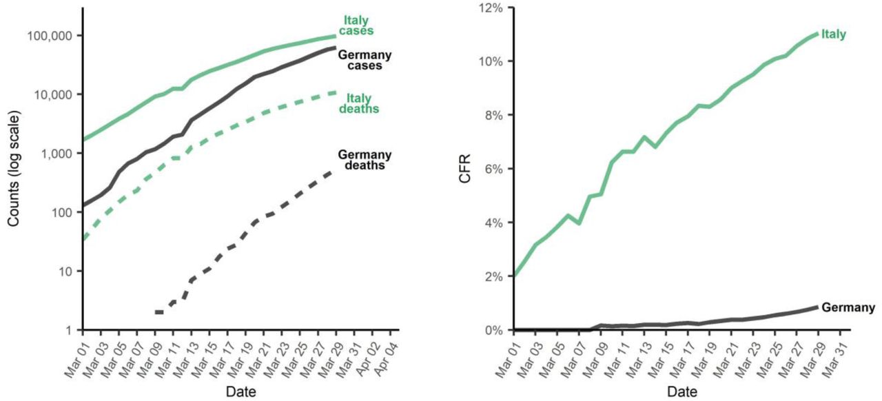
Examples of this discrepancy are shown in Figure 1. As of March 24, 2020, Germany had a total of around 27 thousand confirmed infections and 114 deaths, resulting in a CFR of around 0.4%. Italy, on the other hand, up to the same day, had close to 64 thousand confirmed cases of infection, around 6 thousand deaths, and a CFR of 9.5%. On March 16, Italy had roughly the same number of cases as Germany on March 24, and a CFR of 7.7%. Thus, the outbreak in Italy is going along with a much higher CFR, and the CFR increased over time [2, 3].
(Left panel) COVID-19 confirmed cases and deaths; (right panel) case fatality rates (CFR) in Italy and Germany since March 1 2020.
Differences in the CFR could indicate that the risk of dying of COVID-19 among detected cases differs between countries or changes within a population over time. On the other hand, it could also imply compositional differences in the detected infections [1, 3]. Specifically, the risk of dying of COVID-19 is well-documented to increase with age. Thus, if the population of infected individuals is older in one country or time period than in another, the CFR will be higher, even if the age-specific risk of dying is the same.
Indeed, demographers have argued that age structure matters [4, 5], and the age composition of the reported cases has been suggested as a potential explanation for differences in CFRs [1, 3]. So far, however, there have been no assessments of the importance of the age structure of diagnosed cases versus the age-specific CFR.
In this paper, we analyze cross-country differences in observed CFRs and within-country time trends in CFRs. We use recent data on China, France, Germany, Italy, South Korea, Spain, and the United States. We use a standard demographic decomposition technique [6] to disentangle two potential drivers of differences and trends: (1) the age structure of diagnosed infection cases and (2) age-specific case-fatality rates. We interpret our findings in light of the unfolding knowledge about data-driven biases.
Decomposition approaches like the one used in this paper are commonly used to explain the role of age structure on changing incidence rates [7]. They have also been applied to differences in cancer fatality rates across regions with varying age structures [8]. We are not aware of any application to CFRs of infectious diseases in general and the COVID-19 pandemic in particular.
To facilitate the application of the approach described in this paper, we provide code and reproducibility materials for the open source statistical software R in a freely-accessible repository on the Open Science Framework: https://osf.io/vdgwt/. Moreover, we also provide some examples in an Excel spreadsheet in the same repository.
2 Data and Methods
2.1 Data
We gathered data on the cumulative number of diagnosed infections and deaths attributable to COVID-19 for the following populations (in alphabetical order): China, France, Germany, Italy, South Korea, Spain, the United States (country), and United States (New York City only). An overview of the data is given in Table 1. Countries were included in the analysis based on the availability of case and death counts by age. Unfortunately, many countries do not report breakdowns by age and therefore could not be included in our analysis.
Countries covered in the analysis, and their cumulative detected cases and deaths. For most countries, we use the latest data available to us. For Italy, we also analyze trends over time. The cumulative cases and deaths shown for Italy in this table are for March 29.
All data is provided by the respective health authorities, except for the death data for Germany, which is based on press reports of age at death collected on Wikipedia. A complete list of sources is given in Appendix D.
For some of the countries (Germany, Italy, Spain, and the United States) age is not available for some confirmed cases or deaths. We imputed the missing age using the observed age distribution of cases or deaths, respectively. Removing these cases from the analysis altogether has no substantive impact on the results, except for Spain, where around 40% of cases and 62% of deaths have no recorded age. Ignoring cases and deaths of unknown age in Spain would therefore deflate age-specific case fatality rates.
The original data is provided in different age groupings. For the decomposition, the age groups have to match. We therefore adjusted counts so that all countries conform with the age groups of South Korea, for which the age groups are 10-year age groups from birth to 80+. Counts were split using a recently proposed method tailored for this data situation [9]. Appendix C shows the original age groups of the data.
2.2 Case fatality rates
The COVID-19 case fatality rate (CFR) is defined as the ratio of deaths (D) associated with COVID-19 divided by the number of detected COVID-19 cases (N): CFR=D/N. In our application, the death and case counts are cumulative counts up to a certain date.
If case counts and death counts are available by age, which is our situation, the CFR can also be written as a sum of age-specific CFRs weighted by the proportion of cases in a certain age group. We use a as an index to denote different age groups. These age groups could, for instance, be 0 years to 9 years, 10 years to 19 years, and so on, but other groupings are also possible. We define age-specific CFRs as  i.e., the number of deaths in age group a divided by the number of cases in the same age group. The proportion of cases in age group a is given by
  Using this notation, the CFR can be written as a weighted average of age-specific CFRs:
We use the weighted expression and a mathematical decomposition approach introduced by Kitagawa [Kitagawa] to separate the difference between two CFRs into two distinct parts, one attributable to age-structure and another to age-specific case-fatality. The method attributes the total difference into these two components, leaving no residual. In other words, if we use i and j to index two different populations, then the decomposition approach splits the difference between their CFRs into
 where the α-component captures the effect of the age structure, and the δ-component indicates the part of the difference attributable to age-specific case-fatality. The details of the method are described in Appendix A, which also provides a step-by-step walk-through of the decomposition.
3 Results
3.1 Country comparisons
Table 2 shows results for cross-country comparisons using the data from South Korea (March 26) as a reference, with countries sorted by increasing CFR. We chose South Korea as the reference because its CFR is arguably the closest match to itsactual infection rate due to extensive testing and an earlier onset of the epidemic; moreover, the CFR was comparably low, and decompositions will estimate what factor leads other countries to differ from this low CFR setting, making results easy to interpret. In appendix B, we provide additional results using Germany (lowest CFR) and Italy (highest CFR) as reference countries.
Results of the cross-country decompositions using South Korea as a reference case. The third column shows the difference between each country and South Korea as a reference, and is calculated as the CFR of South Korea minus the CFR of the respective country.
Based on the cumulative data up to March 30, South Korea had a CFR of 1.6% (third line of the table, column CFR). Only Germany and New York City had lower CFRs of 0.7% and 1.2%, respectively. The difference to the South Korean CFR is shown in the third column of the table (South Korea minus Germany or New York City), and is positive, indicating that the South Korean CFR is higher, although the difference is relatively small. The fourth and fifth column of the table show the absolute contributions of the age distribution and age-specific fatality rates, respectively. A negative number for the age structure indicates an older age structure of detected cases compared to South Korea, while a negative number for the fatality rates indicates higher age-specific mortality rates compared to South Korea. The sixth and seventh column of the table indicate the relative contributions of the components; in the case of Germany and New York City, the lower CFR compared to South Korea is largely due to higher survival of reported cases, 96% for both Germany and New York City.
All other countries (the United States, China, France, Spain, and Italy) have a higher CFR than South Korea, as indicated by the negative difference shown in column four of Table 2, and some of the differences are substantial. For instance, the French CFR is more than twice as high as the South Korean, while the Italian is almost seven times as high.
At first glance there is no consistent pattern in the (relative) contributions of the α-component (age) and the δ-component (fatality). For instance, the CFR in China (2.3%) is somewhat lower than the CFR of France (2.6%), and both are one or two percentage points above South Korea. In China 86% of the difference in the CFR to South Korea is explained by higher case fatality, while in France it is largely due to the age structure (89%). In the two cases with the highest CFRs – Italy and Spain – the relative contributions were similar with the α-component explaining more than half of the difference, and the δ-component explaining the remainder.
3.2 Trends over time
The case of Italy
Italy is the only country for which we have a relatively long time series of data spanning several weeks. Table 3 documents how the Italian CFR evolved from March 9 to March 29. The CFR of March 9 is used as a reference, and the decomposition shows which factor is driving the trend in the CFR. From the beginning to the end of the period under study the CFR more than doubled, from 4.3% to 10.6%. This increase over time is largely driven by worsening fatality of COVID-19 – the fatality component explaining more than 95% of the rise in all time periods – and changes in the age structure only played a minor role, with detected cases moving to a more favorable (younger) age distribution and slightly counteracting the effect of worsening fatality. As a robustness check we changed the reference period from March 9 to March 19. This resulted in the fatality component explaining 88% of the increase in CFR.
Development of the Italian CFR over time. The third column gives the difference between the CFR of the respective date minus the CFR of March 9.
4 Discussion
Case fatality rates (CFRs) associated with COVID-19 vary strongly across countries and over time within countries. Our findings show that there is substantial variation in which factor explains the differences in CFRs. Differences in the age distribution of detected infections in some cases explain a substantial part of the total difference in CFRs. In particular, more than 50% of the difference in CFRs between countries with a low CFR and a high CFR can be explained by the age structure of detected infections. In contrast, in the case of Italy we observe a substantial increase in the CFR over time, mostly attributable to increasing age-specific case-fatality.
Ultimately, the approach discussed here does not directly explain why the age structure of confirmed cases or the age-specific fatality rates matter more in one case and less in another, and some expertise about the contexts which are being compared is required to interpret results. We discuss some potential explanations below.
Differences in the age structure of the populations which are being compared are unlikely to be a major driver of the age component that we estimated here, as the age composition of confirmed cases does not necessarily match the age composition of the population. For instance, according to Eurostat, the proportion of the population aged 80+ in 2019 was 7% in Italy and 6.5% in Germany, while in our data the proportion of reported infections in the same age range was close to 20% for Italy and only 4% in Germany.
Differences in testing regimes are a plausible mechanism driving the different detected age structures of cases [3, 10, 11]. This is consistent with our finding that differences between countries with extensive early testing of contacts to known cases (South Korea, Germany) are largely driven by differences in fatality and not by differences in the age distribution, suggesting that those countries might be more successful at catching the mild and asymptomatic cases among the younger population groups. However, it is also plausible that the extensive testing itself in these countries prevented undetected community spread to older population groups. Moreover, the data included in our analysis is also based on extensive testing for Italy and to a lesser extent for Spain, as these countries ramped up testing as the epidemic spread, making test numbers alone an unlikely explanation for the different age structure of detected cases.
Differences in the COVID-19 transmission pathways might also be a factor. Depending on contact patterns and household structure, the elderly population might be affected earlier in some countries than in others, leading to a less favorable age distribution of infections [4, 12]. This could be relevant in explaining why the age distribution plays such a large role for the two countries with by far the highest CFR, Spain and Italy, which have a relatively large proportion of individuals living with their elderly parents or grandparents, and comparatively intensive intergenerational contact [13-15].
The trend over time in the Italian CFR is an example where changes in age-specific fatality rates are driving trends instead of changes in the age distribution. This likely reflects the worsening situation in Italy over time as its health care system got under increasing pressure [16, 10]. However, an increase in CFR could also be expected once containment measures become effective, and newly confirmed cases increase at a slower pace than deaths from cases acquired prior to containment policies.
Only once an epidemic reaches its final conclusion and all cases have either resulted in recovery or fatalities, can the importance of the age difference in cases on CFRs be assessed with an acceptable degree of accuracy [17]. In this context a distinction should be made between CFRs, which are solely based only on detected cases, and infection fatality rates (IFRs) which estimate the risk of dying from all infections, including asymptomatic and undiagnosed cases. Ideally policies for containing the spread of a virus would be designed on the basis of IFRs. However, particularly early on in an epidemic, the CFR is the only metric available until the extent of known data-driven biases can be assessed [1, 10, 11, 18-21].
Data quality can affect both the age composition of detected cases and age-specific fatality rates. For instance, counts may be affected by issues like reporting delays or censoring, or by inconsistent case definitions [1, 2, 18, 19, 22]. Deaths may be underestimated because of lack of testing both before and after death. Countries might also differ in how they code deaths from underlying or contributory causes.
The relative importance of both the case age structure and mortality components could also be affected by comparing countries at different stages of the epidemic. This could result from cases not being detected at the beginning of the epidemic [23], or from differences in the lag between infection and death [22, 10]. Generally, CFRs are highest at the beginning of an outbreak, when the most serious cases are the most readily detected, and declines as testing capacity increases and less serious cases are identified [21], which was notably not the case in Italy.
Finally, the choice of age groups may have affected our results. If ages were grouped too widely it might hide actual age-specific case fatality differences. For instance, if the median age within the 10-year aggregated age groups that we used differed between populations, this would reduce the case-age structure explanation and inflate the age-specific mortality explanation. Finally, there are alternative decomposition techniques that might yield different results. However, differences are expected to be rather small; indeed, applying the method of Horiuchi [24] to our data yields virtually the same results (results available upon request).
The results of this study add weight to recommendations for data to be disaggregated by age and potentially other variables to facilitate a better understanding of population-level differences in CFRs. Equally important will be well designed seroprevalence studies to ascertain the extent to which our findings are driven by differences in testing regimes, particularly in the diagnosis of mild and asymptomatic cases. To this extent we are encouraged by the recent announcement that such a study is being initiated in Germany [25] in line with official WHO recommendations [26].
Overall, our results show that differences between countries with low and high CFRs can be driven to a significant extent by the age structure of cases. Decomposing differences in case fatality rates over time or between countries reveals important insights for monitoring the spread of COVID-19. An accurate assessment of these differences in CFR across countries and over time are crucial to inform and determine appropriate containment and mitigation interventions, such as social confinement and mobility restrictions.
A. Details of the decomposition method
A.1 Decomposing CFRs
We want to decompose, or “explain”, the difference between two CFRs, irrespective of whether they are from two different populations, or from the same population at two different points in time, or from different groups within a population, e.g., gender or socio-economic groups. We will use CFRi and CFRj to distinguish the two CFRs, e.g., country i and country j. Moreover, we write Pia, Cia, Pja, and Cja for the underlying age compositions and age-specific CFRs; i.e., CFRi = ∑PiaCia.
Using a decomposition approach introduced by Kitagawa [6] we separate the difference between two CFRs into two distinct parts,
 where α captures the part of the difference between CFRs which is due to differences in the age composition of cases, and δ is due to differences in mortality.α is given by
 while δ can be calculated as

Note that the age groups for group i and group j need to be the same. If this is not the case in the raw data and, for instance, one country reports counts in 5-year age groups (0-4, 5-9, 10-14, 15-19, …) and the other uses 10-year age groups (0-9, 10-19, …), then either the more finely grained data needs to be aggregated to match the coarser data, or the coarser data needs to be adjusted. We choose the latter approach (see appendix C below).
The intuition behind the formulas is as follows. The first two terms in brackets in the equation for α are CFRi − ∑PjaCia, or, replacing CFRi with its definition, ∑PiaCia − ∑PjaCia. The second sum in this expression captures how high the CFR would have been if group i had the same age distribution of infections as group j. The difference to the actual CFR (the whole expression) then captures to what extent the CFR is higher than this hypothetical CFR because of the actually observed age distribution of detected infections. The third and the fourth term in brackets in the equation for α are following a similar logic, but using a different hypothetical comparison, asking how much the CFR of group j would differ if the detected cases had the age distribution of group i. The formula for δ again follows a similar logic, but now replacing the age-specific CFRs instead of the age distribution. In summary, to decompose the difference between two CFRs requires nothing more than the two CFRs themselves as well as a few additional hypothetical CFRs.
To calculate the proportion α and δ contribute to the total difference one can use  in case of α and
  for the contribution of δ.
A.2 Interpretation
As an artificial example, assume that the CFR in country A is equal to 2 percent, while it equals 4 percent in country B. Subtracting the CFR of country A from country B gives a difference of 2 percentage points. If a large part of this difference is due to the age structure, then α could be 0.015 and δ could be 0.005. These sum to 0.02, or 2 percentage points. If, as another example, two countries have the same age structure of cases, then α will be zero. A similar reasoning holds for δ if age-specific CFRs are the same for both countries being compared. In relative terms, the α-component explains 75 percent of the difference between countries, while the δ-component only explains 25 percent.
The total difference between two CFRs as well as both α and δ can be negative. The formulas for the relative contributions take this into account by using absolute values. If the total difference is positive and either α or δ are negative, it means that the corresponding part of the difference actually reduces the difference between CFRs. For instance, when comparing the CFR for one country at two points in time, the total difference could be 0.03; i.e., the CFR increased by three percentage points. If in this case α would be negative, say −0.01, it would mean that the age distribution of cases over time became more favorable. δ would be 0.04 in this scenario, and without changes in the age distribution of infections as captured through α, the difference between CFRs would even have increased by four percentage points.
B. Additional results
C. Additional information on data: Age groups
The data we use is provided in different age groups, depending on the country. The following age groups are used in the original data for both case counts and death counts:
China: 0-9, 10-19, 20-29, 30-39, 40-49, 50-59, 69-69, 70-79, 80+
France: 0-14, 15-44, 45-64, 65-74, 75+
Germany: 0-4, 5-14, 15-34, 35-59, 60-79, 80+
Italy: 0-9, 10-19, 20-29, 30-39, 40-49, 50-59, 69-69, 70-79, 80-89, 90+
Spain: 0-9, 10-19, 20-29, 30-39, 40-49, 50-59, 69-69, 70-79, 80+
South Korea: 0-9, 10-19, 20-29, 30-39, 40-49, 50-59, 69-69, 70-79, 80+
United States: 0-19, 20-44, 45-54, 55-64, 65-74, 75-84, 85+
United States (New York City): 0-18, 18-44, 45-64, 65-74, 75+
For the decomposition, the age groups have to match. This is the case for China, Spain, South Korea, and Italy; in case of the latter the age categories 80-89 and 90+ have to be merged. The age groups provided for France, Germany, and the United States are problematic, as they do not match the age groups of any other country. Aggregating the age groups, as for Italy, does not help, either. For instance, the age category of 15 years to 44 years available for France cannot be created based on the German data. To deal with this issue, we adjusted the case counts and death counts for France, Germany, and the United States using a smoothing approach, which is able to estimate counts for age groups 0-9, 10-19, …, 80+ [9].
D. Data sources
A spreadsheet containing all data we used, as well as data for additional countries and dates is available at https://osf.io/vdgwt/ as part of our materials for reproducibility.
A complete list of sources for that data, including date of access, is provided here: https://github.com/timriffe/covid_demog/blob/master/sources/sources.md
Below is the list of sources used for our main analyses:
https://www.cdc.go.kr/board/board.es?mid=a30402000000&bid=0030&act=view&list_no366578
https://experience.arcgis.com/experience/478220a4c454480e823b17327b2bf1d4
https://www.cdc.gov/mmwr/volumes/69/wr/mm6912e2.htm?s_cid=mm6912e2_w#T1_down https://www1.nyc.gov/assets/doh/downloads/pdf/imm/covid-19-daily-data-summary.pdf
E. Excel spreadsheet and R code
All R code used to produce the results in the paper as well as the data can be downloaded from https://osf.io/vdgwt/. An Excel spreadsheet containing several examples can be found in the same repository.
Footnotes
riffe{at}demogr.mpg.de, vanraalte{at}demogr.mpg.de, acosta{at}demogr.mpg.de, myrskyla{at}demogr.mpg.de
References


