
Abstract
Governments around the world are responding to the novel coronavirus (COVID-19) pandemic1 with unprecedented policies designed to slow the growth rate of infections. Many actions, such as closing schools and restricting populations to their homes, impose large and visible costs on society. In contrast, the benefits of these policies, in the form of infections that did not occur, cannot be directly observed and are currently understood through process-based simulations.2–4 Here, we compile new data on 1,659 local, regional, and national anti-contagion policies recently deployed in the ongoing pandemic across localities in China, South Korea, Iran, Italy, France, and the United States (US). We then apply reduced-form econometric methods, commonly used to measure the effect of policies on economic growth, to empirically evaluate the effect that these anti-contagion policies have had on the growth rate of infections. In the absence of any policy actions, we estimate that early infections of COVID-19 exhibit exponential growth rates of roughly 42% per day. We find that anti-contagion policies collectively have had significant effects slowing this growth. Our results suggest that similar policies may have different impacts on different populations, but we obtain consistent evidence that the policy packages now deployed are achieving large, beneficial, and measurable health outcomes. We estimate that, to date, current policies have already prevented or delayed on the order of 62 million infections across these six countries. These findings may help inform whether or when these ongoing policies should be lifted or intensified, and they can support decision-making in the other 180+ countries where COVID-19 has been reported.5
Introduction
The 2019 novel coronavirus1 (COVID-19) pandemic is forcing societies around the world to make consequential policy decisions with limited information. After containment of the initial outbreak failed, attention turned to implementing large-scale social policies designed to slow contagion of the virus,6 with the ultimate goal of slowing the rate at which life-threatening cases emerge so as to not exceed the capacity of existing medical systems. In general, these policies aim to decrease opportunities for virus transmission by reducing contact among individuals within or between populations, such as by closing schools, limiting gatherings, and restricting mobility. Such actions are not expected to halt contagion completely, but instead are meant to slow the spread of COVID-19 to a manageable rate. These large-scale policies are informed by epidemiological simulations2, 4, 7–17 and a small number of natural experiments in past epidemics.18 However, the actual effects of these policies on infection rates in the ongoing pandemic are unknown. Because the modern world has never experienced a pandemic from this pathogen, nor deployed anti-contagion policies of such scale and scope, it is crucial that direct measurements of policy impacts be used alongside numerical simulations in current decision-making.
Populations across the globe are currently weighing whether, or when, the health benefits of anti-contagion policies are worth the costs they impose on society. Many of these costs are plainly seen; for example, restrictions imposed on businesses are increasing unemployment,19 travel bans are bankrupting airlines,20 and school closures may have enduring impacts on affected students.21 It is therefore not surprising that some populations hesitate before implementing such dramatic policies, particularly when these costs are visible while their health benefits – infections and deaths that would have occurred but instead were avoided or delayed – are unseen. Our objective is to measure the direct health benefits of these policies; specifically, how much these policies slowed the growth rate of infections. We treat recently implemented policies as hundreds of different natural experiments proceeding in parallel. Our hope is to learn from the recent experience of six countries where early spread of the virus triggered large-scale policy actions, in part so that societies and decision-makers in the remaining 180+ countries can access this information.
Here we directly estimate the effects of 1,659 local, regional, and national policies on the growth rate of infections across localities within China, France, Iran, Italy, South Korea, and the US (see Figure 1 and Supplementary Table 1). We compile publicly available subnational data on daily infection rates, changes in case definitions, and the timing of policy deployments, including (1) travel restrictions, (2) social distancing through cancellations of events and suspensions of educational/commercial/religious activities, (3) quarantines and lockdowns, and (4) additional policies such as emergency declarations and expansions of paid sick leave, from the earliest available dates to April 6, 2020 (see complete descriptions in the Supplementary Information, also Extended Data Fig. 1). During this period, populations in these countries remained almost entirely susceptible to COVID-19, causing the natural spread of infections to exhibit almost perfect exponential growth.7, 14, 22 The rate of this exponential growth may change daily and is determined by epidemiological factors, such as disease infectivity and contact networks, as well as policies that induce behavior changes.7, 8, 22 We cannot experimentally manipulate policies ourselves, but because they are being deployed while the epidemic unfolds, we can estimate their effects empirically. We examine how the daily growth rate of infections in each locality changes in response to the collection of ongoing policies applied to that locality on that day.

The left-hand-side plots show daily cumulative confirmed cases of COVID-19 (solid black line) and deaths (dashed black line) over time (left axis for both). Deployment of anti-contagion policies are indicated by vertical lines, with height corresponding to the number of administrative units that instituted the policy on a given day (right axis). For display purposes only, not all policies are shown for each country (≤ 5 types highlighted per country) and cases are imputed for days with missing data. The right-hand-side maps show the number of cumulative confirmed cases by administrative unit on the last date of each sample (circle area = number of cases).
We employ well-established “reduced-form” econometric techniques23, 24 commonly used to measure the effects of policies25, 26 or other events (e.g., wars27 or environmental changes28) on economic growth rates. Similarly to early COVID-19 infections, economic output generally increases exponentially with a variable rate that can be affected by policies and other conditions. Unlike process-based epidemiological models,7–9, 12, 22, 29, 30 the reduced-form statistical approach to inference that we apply does not require explicit prior information about fundamental epidemiological parameters or mechanisms, many of which remain uncertain in the current pandemic. Rather, the collective influence of these factors is empirically recovered from the data without modeling their individual effects explicitly (see Methods). Prior work on influenza,31 for example, has shown that such statistical approaches can provide important complementary information to process-based models.
To construct the dependent variable, we transform location-specific, subnational time-series data on infections into first-differences of their natural logarithm, which is the per-day growth rate of infections (see Methods). We use data from first- or second-level administrative units and data on active or cumulative cases, depending on availability (see Supplementary Information). We then employ widely-used panel regression models23, 24 to estimate how the daily growth rate of infections changes over time within a location when different combinations of large-scale social policies are enacted (see Methods). Our econometric approach accounts for differences in the baseline growth rate of infections across sub-national locations, which may be affected by time-invariant characteristics, such as demographics, socio-economic status, culture, and health systems; it accounts for systematic patterns in growth rates within countries unrelated to policy, such as the effect of the work-week; it is robust to systematic under-surveillance specific to each sub-national unit; and it accounts for changes in procedures to diagnose positive cases (see Methods and Supplementary Information). The reduced-form statistical techniques we use are designed to measure the total magnitude of the effect of changes in policy, without attempting to explain the origin of baseline growth rates or the specific epidemiological mechanisms linking policy changes to infection growth rates (see Methods). Thus, this approach does not provide the important mechanistic insights generated by process-based models; however, it does effectively quantify the key policy-relevant relationships of interest using recent real-world data, when fundamental epidemiological parameters are still uncertain.
Results
We estimate that in the absence of policy, early infection rates of COVID-19 grow 42% per day on average (Standard Error [SE] = 7%), implying a doubling time of approximately 2 days. Country-specific estimates range from 24% per day in China (SE = 9%) to 69% per day in Iran (SE = 5%). Growth rates in South Korea, Italy, France, and the US are very near the 42% average value (Figure 2a). These estimated values differ from observed growth rates because the latter are confounded by the effects of policy. These growth rates are not driven by the expansion of testing or increasing rates of case detection (see Methods and Extended Data Fig. 2) and are not dependent on data from any particular region of any country (Extended Data Fig. 3).

Markers are country-specific estimates, whiskers are 95% CI. Columns report effect sizes as a change in the continuous-time growth rate (95% CI in parentheses) and the day-over-day percentage growth rate. (a) Estimates of daily COVID-19 infection growth rate in the absence of policy (red dashed line = average, excluding Wuhan-specific estimate). (b) Estimated combined effect of all policies on infection growth rates. (c) Estimated effects of individual policies or policy groups on the daily growth rate of infections, jointly estimated.
Some prior analyses of pre-intervention infections in Wuhan suggest slower growth rates (doubling every 5–7 days)32, 33 using data collected before national standards for diagnosis and case definitions were first issued by the Chinese government on January 15, 2020.34 However, case data in Wuhan from before this date contains multiple irregularities:34 the cumulative case count decreased on January 9; no new cases were reported between January 9 and January 15; and there were concerns over whether information about the outbreak was actively suppressed35 (see Supplementary Table 2). When we remove these problematic data, utilizing a shorter but more reliable pre-intervention time series from Wuhan (January 16–21, 2020), we recover a growth rate of 43% per day (SE = 3%, doubling every 2 days) consistent with results from all other countries (Figure 2a and Supplementary Table 3), except Iran.
During the early stages of an epidemic, a large proportion of the population remains susceptible to the virus, and if the spread of the virus is left uninhibited by policy or behavioral change, exponential growth will continue until the fraction of the susceptible population declines meaningfully.7, 29 This decline results from members of the population leaving the transmission cycle, due to either recovery or death.29 After correcting for estimated rates of case-detection,36 we compute that the minimum susceptible population in any of the administrative units in our sample is approximately 78.0% of the total population (Cremona, Italy: roughly 79,000 total infections in a population of 360,000) and 86% of administrative units across all six countries would likely be in a regime of uninhibited exponential growth (susceptible fraction of population > 95%) if policies were removed on the last date of our sample.
Consistent with predictions from epidemiological models,2, 18, 37 we find that the combined effect of policies within each country reduces the growth rate of infections by a substantial and statistically significant amount (Figure 2b, Supplementary Table 3). For example, a locality in France with a baseline growth rate of 0.34 (national average) that fully deployed all policy actions used in France would be expected to lower its daily growth rate by −0.28 to a growth rate of 0.06. In general, the estimated total effects of policy packages are large enough that they can in principle offset a large fraction of, or even eliminate, the baseline growth rate of infections—although in several countries, many localities are not currently deploying the full set of policies used in that country. Overall, the estimated effects of all policies combined are generally insensitive to dropping regional (i.e. state- or province-level) blocks of data from the sample (Extended Data Fig. 3).
In China, only two policies were enacted across 116 cities early in a seven week period, providing us with sufficient data to empirically estimate how the effects of these policies evolve over time without making any assumptions about the timing of these effects (see Methods and Fig. 2b). We estimate that the combined effect of these policies significantly reduced the growth rate of infections by −0.14 (SE = 0.031) in the first week immediately following their deployment (also see Extended Data Fig. 5a), with effects doubling in the second week to −0.30 (SE = 0.040), and stabilizing in the third week at −0.34 (SE = 0.036). In other countries, we lack sufficient data to estimate these temporal dynamics explicitly and only report the average pooled effect of policies across all days following their deployment (see Methods). If other countries were to exhibit transient responses similar to that observed in China, we would expect effects in the first week following deployment to be smaller in magnitude than the average effect for all post-deployment weeks. Below, we explore how our estimates would change if we impose the assumption that policies cannot affect infection growth rates until after a fixed number of days, but we do not find evidence this improves model fit (Extended Data Fig. 5b).
The estimates described above (Figure 2b) capture the superposition of all policies deployed in each country, i.e., they represent the average effect of policies on infection growth rates that we would expect to observe if all policies enacted anywhere in each country were implemented simultaneously in a region of that country. We also estimate the effects of individual policies or clusters of policies that are grouped either based on their similarity in goal (e.g., library closures and museum closures are grouped) or timing (e.g., policies that are generally deployed simultaneously in a certain country). In many cases, our estimates for these effects are statistically noisier than the estimates for all policies combined because we are estimating multiple effects simultaneously. Thus, we are less confident in the individual estimates and in their relative rankings. Estimated effects differ between countries, and policies are neither identical nor perfectly comparable in their implementation across countries or, in many cases, across different localities within the same country. Nonetheless, despite a higher level of variability in these values, 28 out of 34 point estimates indicate that individual policies are likely contributing to reducing the growth rate of infections (Figure 2c). Six policies (one in South Korea, two in Italy, and three in the US) have point estimates that are positive, five of which are small in magnitude (< 0.1) and not statistically different from zero (5% level). Consistent with greater overall uncertainty in these dis-aggregated estimates, some in China, France, Italy, and South Korea are somewhat more sensitive to dropping regional blocks of data (Extended Data Fig. 4). The estimated effects of individual policies are broadly robust to assuming a constant delayed effect of all policies (Extended Data Fig. 5c).
We combine the estimates above with our data on the timing of the 1,659 policy deployments to estimate the total effect of all policies across the dates in our sample. To do this, we use our estimates to predict the growth rate of infections in each locality on each day, given the policies in effect at that location on that date (Figure 3, blue markers). We then use the same model to predict what counterfactual growth rates would be on that date if all policies were removed (Figure 3, red markers), which we refer to as a “no-policy scenario.” The difference between these two predictions is our estimated effect that all anti-contagion policies actually deployed had on the growth rate of infections. We estimate that since the beginning of our sample, on average, all anti-contagion policies combined have slowed the average daily growth rate of infections by −0.156 per day (±0.015, p < 0.001) in China, −0.248 (±0.089, p < 0.001) in South Korea, −0.241 (±0.068, p < 0.001) in Italy, −0.362 (±0.069, p < 0.001) in Iran, −0.139 (±0.038, p < 0.001) in France and −0.092 (±0.033, p < 0.05) in the US. Taken together, these results suggest that anti-contagion policies currently deployed in all six countries are achieving their intended objective of slowing the pandemic, broadly confirming epidemiological simulations. These results are robust to modeling the effects of policies without grouping them (Extended Data Fig. 6a and Supplementary Table 4) or assuming a delayed effect of policy on infection growth rates (Supplementary Table 5). At a particular moment in time, the total number of COVID-19 infections depends on the growth rate of infections on all prior days. Thus, persistent decreases in growth rates have a compounding effect on total infections, at least until a shrinking susceptible population slows growth through a different mechanism. To provide a sense of scale and context for our main results in Figs. 2 and 3, we integrate the growth rate of infections in each locality from Figure 3 to estimate the total number of infections to date, both with actual anti-contagion policies and in the no-policy counterfactual scenario. To account for the declining size of the susceptible population in each administrative unit, we couple our econometric estimates of the effects of policies with a simple Susceptible-Infected-Removed (SIR) model of infectious disease dynamics7, 22 that adjusts the susceptible population based on previously estimated case-detection rates36 (see Methods). This allows us to extend our projections beyond the initial exponential growth phase of infections, a threshold which our results suggest would currently be exceeded in several countries in the no-policy scenario.

Predicted daily growth rates of active (China and South Korea) or cumulative (all others) COVID-19 infections based on the observed timing of all policy deployments within each country (blue) and in a scenario where no policies were deployed (red). The difference between these two predictions is our estimated effect of actual anti-contagion policies on the growth rate of infections. Small markers are daily estimates for subnational administrative units (vertical lines are 95% CI). Large markers are national averages. Black circles are observed daily changes in log(infections), averaged across administrative units.
Our results suggest that ongoing anti-contagion policies have already substantially reduced the number of COVID-19 infections observed in the world today (Figure 4). Our central estimates suggest that there would be roughly 27 million more cumulative confirmed cases in China, 20 million more in South Korea, 2.7 million more in Italy, 5.4 million more in Iran, 530,000 more in France, and 5.1 million more in the US had these countries never enacted any anti-contagion policies since the start of the pandemic. The relative magnitudes of these impacts partially reflects the timing, intensity, and extent of policy deployment (e.g., how many localities deployed policies), and the duration for which they have been applied. Several of these estimates are subject to large statistical uncertainties (see intervals in Figure 4). Sensitivity tests that assume a range of plausible alternative parameter values and disease dynamics, such as incorporating a Susceptible-Exposed-Infected-Removed (SEIR) model, suggest that policies may have reduced the number of infections by a total of 57–65 million confirmed cases over the dates in our sample (central estimates).

The predicted cumulative number of confirmed COVID-19 infections based on actual policy deployments (blue) and in the no-policy counterfactual scenario (red). Shaded areas show uncertainty based on 1,000 simulations where empirically estimated parameters are resampled from their joint distribution (dark = inner 70% of predictions; light = inner 95%). Black dotted line is observed cumulative infections. Infections are not projected for administrative units that never report infections in the sample, but which might have experienced infections in a no-policy scenario.
Discussion
Overall, our results indicate that large-scale anti-contagion policies are achieving their intended objective of slowing the growth rate of COVID-19 infections. Because infection rates in the countries we study would have initially followed rapid exponential growth had no policies been applied, our results suggest that these ongoing policies are currently providing large health benefits. For example, we estimate that there would be roughly 339× the current number of confirmed infections in China, 22× in Italy, and 15× in the US by the end of our sample if large-scale anti-contagion policies had not already been deployed. Consistent with process-based simulations of COVID-19 infections,2, 4, 10–12, 14, 17, 29 our empirical analysis of existing policies indicates that seemingly small delays in policy deployment likely produce dramatically different health outcomes.
While the limited amount of currently available data poses challenges to our analysis, our aim is to use what data exist to estimate the first-order impacts of unprecedented policy actions in an ongoing global crisis. As more data become available, empirical research findings will become more precise and may capture more complex interactions. For example, this analysis does not account for potentially important interactions between populations in nearby localities,7, 38 nor the structure of mobility networks.3, 4, 10, 12, 17, 39 Nonetheless, we hope the results we are able to obtain at this early stage of the pandemic can support critical decision-making, both in the countries we study and in the other 180+ countries where COVID-19 infections have been reported.
A key advantage of our reduced-form “top down” statistical approach is that it captures the real-world behavior of affected populations without requiring that we explicitly model all underlying mechanisms and processes. This property is useful in the current stage of the pandemic when many process-related parameters remain unknown. However, our results cannot and should not be interpreted as a substitute for process-based epidemiological models specifically designed to provide guidance in public health crises. Rather, our results complement existing models, for example, by helping to calibrate key model parameters. We believe both forward-looking simulations and backward-looking empirical evaluations should be used to inform decision-making.
Our analysis measures changes in local infection growth rates associated with changes in anti-contagion policies, treating each subnational administrative unit as if it were in a natural experiment. Intuitively, each administrative unit observed just prior to a policy deployment serves as the “control” for the same unit in the days after it receives a policy “treatment”. Thus, a necessary condition for our estimates to be interpreted as the plausibly causal effect of these policies is that the timing of policy deployment is independent of infection growth rates.23 Such an assumption is supported by epidemiological theory, which predicts that infection totals in the absence of policy will be near-perfectly exponential early in the epidemic,7 implying that pre-policy infection growth rates in this context should be constant. The policies we analyze are unlikely to have been deployed in reaction to or anticipation of changes in growth rates, since epidemiological guidance to decision-makers explicitly projected constant growth rates in the absence of anti-contagion measures.2, 29, 40, 41 In practice, decision-makers have tended to deploy policies in response to the count of total infections in their locality, rather than their growth rate,2 in response to outbreaks in other regions or countries,42 or based on other arbitrary and exogenous factors, such as closing schools on a Monday or after Spring Break.43
Our analysis accounts for documented changes in the availability of and procedures for testing for COVID-19 as well as differences in case-detection across locations; however, unobserved trends in case-detection could affect our results (see Methods). For example, if growing awareness of COVID-19 caused an increasing fraction of infected individuals to be tested over time, then unadjusted infection growth rates later in our sample would be biased upwards. Because an increasing number of policies are active later in these samples as well, this bias would cause our current findings to understate the overall effectiveness of anti-contagion policies. However, our analysis of estimated case-detection trends36 (Extended Data Fig. 2) suggests that the magnitude of this potential bias is small, elevating our estimated no-policy growth rates by 0.022 (6%) on average.
It is also possible that changing public information during the period of our study has some unknown effect on our results. If individuals alter their behavior in response to new information unrelated to anti-contagion policies, such as news reports about COVID-19, this could alter the growth rate of infections and thus affect our estimates. Because the quantity of new information is increasing over time, if this information reduces infection growth rates, it would cause us to overstate the effectiveness of anti-contagion policies. We note, however, that if public information is increasing in response to policy actions, then it should be considered a pathway through which policies alter infection growth, not a form of bias. Investigating these potential effects is beyond the scope of this analysis, but it is an important topic for future investigations.
While our analysis has focused on changes in the growth rate of infections, other outcomes, such as hospitalizations or deaths, are also of policy interest. Because these outcomes are more context- and state-dependent than infection growth rates, their analysis in future work may require additional modeling approaches. Nonetheless, we experimentally implement our approach on the daily growth rate of hospitalizations in France, the only country in our sample where we were able to obtain hospitalization data at the granularity of this study. We find that the total estimated effect of anti-contagion policies on the growth rate of hospitalizations is similar to our reported effect on the infection growth rate (Extended Data Fig. 6c).
Here we exclusively analyzed large-scale anti-contagion social policies to understand their effects on infection growth rates within a locality. However, contact tracing, international travel restrictions, and medical resource management, along with many other policy decisions, will play key roles in the global response to COVID-19. Our results do not speak to the efficacy of these other policies.
Lastly, the results presented here are not sufficient on their own to determine which anti-contagion policies are ideal for particular populations, nor do they speak to whether the social costs of individual policies are larger or smaller than the social value of their health benefits. Computing a full value of health benefits also requires understanding how different growth rates of infections and total active infections affect mortality rates, as well as determining a social value for all of these impacts. Furthermore, this analysis does not quantify the sizable social costs of anti-contagion policies, a critical topic for future investigations.
Data Availability
All data and code used in this analysis are available at https://github.com/bolliger32/gpl-covid. Updates are posted at http://www.globalpolicy.science/covid19.
Methods
Data Collection and Processing
We provide a brief summary of our data collection processes here (see the Supplementary Notes for more details, including access dates). Epidemiological, case definition/testing regime, and policy data for each of the six countries in our sample were collected from a variety of in-country data sources, including government public health websites, regional newspaper articles, and crowd-sourced information on Wikipedia. The availability of epidemiological and policy data varied across the six countries, and preference was given to collecting data at the most granular administrative unit level. The country-specific panel datasets are at the region level in France, the state level in the US, the province level in South Korea, Italy and Iran, and the city level in China. Due to data availability, the sample dates differ across countries: in China we use data from January 16 - March 5, 2020; in South Korea from February 17 - April 6, 2020; in Italy from February 26 - April 6, 2020; in Iran from February 27 - March 22, 2020; in France from February 29 - March 25, 2020; and in the US from March 3 - April 6, 2020. Below, we describe our data sources.
China
We acquired epidemiological data from an open source GitHub project1 that scrapes time series data from Ding Xiang Yuan. We extended this dataset back in time to January 10, 2020 by manually collecting official daily statistics from the central and provincial (Hubei, Guangdong, and Zhejiang) Chinese government websites. We compiled policies by collecting data on the start dates of travel bans and lockdowns at the city-level from the “2020 Hubei lockdowns” Wikipedia page2, the Wuhan Coronavirus Timeline project on Github,3 and various other news reports. We suspect that most Chinese cities have implemented at least one anti-contagion policy due to their reported trends in infections; as such, we dropped cities where we could not identify a policy deployment date to avoid miscategorizing the policy status of these cities. Thus our results are only representative for the sample of 116 cities for which we obtained policy data.
South Korea
We manually collected and compiled the epidemiological dataset in South Korea, based on provincial government reports, policy briefings, and news articles. We compiled policy actions from news articles and press releases from the Korean Centers for Disease Control and Prevention (KCDC), the Ministry of Foreign Affairs, and local governments’ websites.
Iran
We used epidemiological data from the table “New COVID-19 cases in Iran by province”4 in the “2020 coronavirus pandemic in Iran” Wikipedia article, which were compiled from the data provided on the Iranian Ministry of Health website (in Persian). We relied on news media reporting and two timelines of pandemic events in Iran5,6 to collate policy data.
Italy
We used epidemiological data from the GitHub repository7 maintained by the Italian Department of Civil Protection (Dipartimento della Protezione Civile). For policies, we primarily relied on the English version of the COVID-19 dossier “Chronology of main steps and legal acts taken by the Italian Government for the containment of the COVID-19 epidemiological emergency” written by the Dipartimento della Protezione Civile,8 and Wikipedia.9
France
We used the region-level epidemiological dataset provided by France’s government website10 and supplemented it with numbers of confirmed cases by region on France’s public health website, which was previously updated daily through March 25.11 We obtained data on France’s policy response to the COVID-19 pandemic from the French government website,12 press releases from each regional public health site,13 and Wikipedia.14
United States
We used state-level epidemiological data from usafacts.org,15 which they compile from multiple sources. For policy responses, we relied on a number of sources, including the U.S. Centers for Disease Control (CDC), the National Governors Association, as well as various executive orders from county- and city-level governments, and press releases from media outlets.
Policy Data
Policies in administrative units were coded as binary variables, where the policy was coded as either 1 (after the date that the policy was implemented, and before it was removed) or 0 otherwise, for the affected administrative units. When a policy only affected a fraction of an administrative unit (e.g., half of the counties within a state), policy variables were weighted by the percentage of people within the administrative unit who were treated by the policy. We used the most recent population estimates we could find for countries’ administrative units (see the Population Data section in the Appendix). Additionally, in order to standardize policy types across countries, we mapped each country-specific policy to one of the broader policy category variables in our analysis. In this exercise, we collected 137 policies for China, 59 for South Korea, 215 for Italy, 22 for Iran, 59 for France, and 1167 for the United States (see Supplementary Table 1).
Epidemiological Data
We collected information on cumulative confirmed cases, cumulative recoveries, cumulative deaths, active cases, and any changes to domestic COVID-19 testing regimes, such as case definitions or testing methodology. For our regression analysis (Figure 2), we use active cases when they are available (for China and South Korea) and cumulative confirmed cases otherwise. We document quality control steps in the Appendix. Notably, for China and South Korea we acquired more granular data than the data hosted on the John Hopkins University (JHU) interactive dashboard;16 we confirm that the number of confirmed cases closely match between the two data sources (see Extended Data Fig. 1). To conduct the econometric analysis, we merge the epidemiological and policy data to form a single data set for each country.
Econometric analysis
Reduced-Form Approach
The reduced-form econometric approach that we apply here is a “top down” approach that describes the behavior of aggregate outcomes y in data (here, infection rates). This approach can identify plausibly causal effects23, 24 induced by exogenous changes in independent policy variables z (e.g., school closure) without explicitly describing all underlying mechanisms that link z to y, without observing intermediary variables x (e.g., behavior) that might link z to y, or without other determinants of y unrelated to z (e.g., demographics), denoted w. Let f (·) describe a complex and unobserved process that generates infection rates y:

Process-based epidemiological models aim to capture elements of f (·) explicitly, and then simulate how changes in z, x, or w affect y. This approach is particularly important and useful in forward-looking simulations where future conditions are likely to be different than historical conditions. However, a challenge faced by this approach is that we may not know the full structure of f (·), for example if a pathogen is new and many key biological and societal parameters remain uncertain. Crucially, we may not know the effect that large-scale policy (z) will have on behavior (x(z)) or how this behavior change will affect infection rates (f (·)).
Alternatively, one can differentiate Equation 1 with respect to the kth policy zk:
 which describes how changes in the policy affects infections through all N potential pathways mediated by x1, …, xN. Usefully, for a fixed population observed over time, empirically estimating an average value of the local derivative on the left-hand-side in Equation 2 does not depend on explicit knowledge of w. If we can observe y and z directly and estimate changes over time
  with data, then intermediate variables x also need not be observed nor modeled. The reduced-form econometric approach23, 24 thus attempts to measure
  directly, exploiting exogenous variation in policies z.
Model
Active infections grow exponentially during the initial phase of an epidemic, when the proportion of immune individuals in a population is near zero. Assuming a simple Susceptible-Infected-Recovered (SIR) disease model (e.g., ref. [22]), the growth in infections during the early period is
 where It is the number of infected individuals at time t, β is the transmission rate (new infections per day per infected individual), γ is the removal rate (proportion of infected individuals recovering or dying each day) and S is the fraction of the population susceptible to the disease. The second equality holds in the limit S→ 1, which describes the current conditions during the beginning of the COVID-19 pandemic. The solution to this ordinary differential equation is the exponential function
 where
where  is the initial condition. Taking the natural logarithm and rearranging, we have

Anti-contagion policies are designed to alter g, through changes to β, by reducing contact between susceptible and infected individuals. Holding the time-step between observations fixed at one day (t2− t1 = 1), we thus model g as a time-varying outcome that is a linear function of a time-varying policy
 where θ0 is the average growth rate absent policy, policyt is a binary variable describing whether a policy is deployed at time t, and θ is the average effect of the policy on growth rate g over all periods subsequent to the policy’s introduction, thereby encompassing any lagged effects of policies. ϵt is a mean-zero disturbance term that captures inter-period changes not described by policyt. Using this approach, infections each day are treated as the initial conditions for integrating Equation 4 through to the following day.
We compute the first differences log(It) − log(It−1) using active infections where they are available, otherwise we use cumulative infections, noting that they are almost identical during this early period (except in China, where we use active infections). We then match these data to policy variables that we construct using the novel data sets we assemble and apply a reduced-form approach to estimate a version of Equation 6, although the actual expression has additional terms detailed below.
Estimation
To estimate a multi-variable version of Equation 6, we estimate a separate regression for each country c. Observations are for subnational units indexed by i observed for each day t. Because not all localities began testing for COVID-19 on the same date, these samples are unbalanced panels. To ensure data quality, we restrict our analysis to localities after they have reported at least ten cumulative infections.
We estimate a multiple regression version of Equation 6 using ordinary least squares. We include a vector of subnational unit-fixed effects θ0 (i.e., varying intercepts captured as coefficients to dummy variables) to account for all time-invariant factors that affect the local growth rate of infections, such as differences in demographics, socio-economic status, culture, and health systems.24 We include a vector of day-of-week-fixed effects d to account for weekly patterns in the growth rate of infections that are common across locations within a country, however, in China, we omit day-of-week effects because we find no evidence they are present in the data – perhaps due to the fact that the outbreak of COVID-19 began during a national holiday and workers never returned to work. We also include a separate single-day dummy variable each time there is an abrupt change in the availability of COVID-19 testing or a change in the procedure to diagnose positive cases. Such changes generally manifest as a discontinuous jump in infections and a re-scaling of subsequent infection rates (e.g., See China in Figure 1), effects that are flexibly absorbed by a single-day dummy variable because the dependent variable is the first-difference of the logarithm of infections. We denote the vector of these testing dummies µ.
Lastly, we include a vector of Pc country-specific policy variables for each location and day. These policy variables take on values between zero and one (inclusive) where zero indicates no policy action and one indicates a policy is fully enacted. In cases where a policy variable captures the effects of collections of policies (e.g., museum closures and library closures), a policy variable is computed for each, then they are averaged, so the coefficient on this type of variable is interpreted as the effect if all policies in the collection are fully enacted. There are also instances where multiple policies are deployed on the same date in numerous locations, in which case we group policies that have similar objectives (e.g., suspension of transit and travel ban, or cancelling of events and no gathering) and keep other policies separate (i.e., business closure, school closure). The grouping of policies is useful for reducing the number of estimated parameters in our limited sample of data, allowing us to examine the impact of subsets of policies (e.g. Fig. 2c). However, policy grouping does not have a material impact on the estimated effect of all policies combined nor on the effect of actual policies, which we demonstrate by estimating a regression model where no policies are grouped and these values are recalculated (Supplementary Table 4, Extended Data Fig. 6).
In some cases (for Italy and the US), policy data is available at a more spatially granular level than infection data (e.g., city policies and state-level infections in the US). In these cases, we code binary policy variables at the more granular level and use population-weights to aggregate them to the level of the infection data. Thus, policy variables may take on continuous values between zero and one, with a value of one indicating that the policy is fully enacted for the entire population. Given the limited quantity of data currently available, we use a parsimonious model that assumes the effects of policies on infection growth rates are approximately linear and additively separable. However, future work that possesses more data may be able to identify important nonlinearities or interactions between policies.
For each country, our general multiple regression model is thus
 where observations are indexed by country c, subnational unit i, and day t. The parameters of interest are the country-by-policy specific coefficients θcp. We display the estimated residuals ϵcit in Extended Data Fig. 10, which are mean zero but not strictly normal (normality is not a requirement of our modeling and inference strategy), and we estimate uncertainty over all parameters by calculating our standard errors robust to error clustering at the day level.23 This approach allows the covariance in ϵcit across different locations within a country, observed on the same day, to be nonzero. Such clustering is important in this context because idiosyncratic events within a country, such as a holiday or a backlog in testing laboratories, could generate nonuniform country-wide changes in infection growth for individual days not explicitly captured in our model. Thus, this approach non-parametrically accounts for both arbitrary forms of spatial auto-correlation or systematic misreporting in regions of a country on any given day (we note that it generates larger estimates for uncertainty than clustering by i). When we report the effect of all policies combined (e.g., Figure 2b) we are reporting the sum of coefficient estimates for all policies
  , accounting for the covariance of errors in these estimates when computing the uncertainty of this sum.
Note that our estimates of θ and θ0 in Equation 7 are robust to systematic under-reporting of infections, a major concern in the ongoing pandemic, due to the construction of our dependent variable. This remains true even if different localities have different rates of under-reporting, so long as the rate of under-reporting is relatively constant. To see this, note that if each locality i has a medical system that reports only a fraction ψi of infections such that we observe Ĩit = ψiIit rather an actual infections Iit, then the left-hand-side of Equation 7 will be
 and is therefore unaffected by location-specific and time-invariant under-reporting. Thus systematic under-reporting does not affect our estimates for the effects of policy θ. As discussed above, potential biases associated with non-systematic under-reporting resulting from documented changes in testing regimes over space and time are absorbed by region-day specific dummies µ.
However, if the rate of under-reporting within a locality is changing day-to-day, this could bias infection growth rates. We estimate the magnitude of this bias (see Extended Data Fig. 2), and verify that it is quantitatively small. Specifically, if Ĩit = ψitIit where ψit changes day-to-day, then
 where log(ψit) − log(ψi,t−1) is the day-over-day growth rate of the case-detection probability. Disease surveillance has evolved slowly in some locations as governments gradually expand testing, which would cause ψit to change over time, but these changes in testing capacity do not appear to significantly alter our estimates of infection growth rates. In Extended Data Fig. 2, we show one set of epidemiological estimates36 for log(ψit) − log(ψi,t−1). Despite random day-to-day variations, which do not cause systematic biases in our point estimates, the mean of log(ψit) − log(ψi,t−1) is consistently small across the different countries: 0.047 in China, 0.066 in Iran, 0.008 in South Korea, 0.053 in France, 0.028 in Italy, and 0.036 in the US. The average of these estimates is 0.022, potentially accounting for 6.2% of our global average estimate for the no-policy infection growth rate (0.35). These estimates of log(ψit) − log(ψi,t−1) also do not display strong temporal trends, alleviating concerns that time-varying under-reporting generates sizable biases in our estimated effects of anti-contagion policies.
Transient dynamics
In China, we are able to examine the transient response of infection growth rates following policy deployment because only two policies were deployed early in a seven-week sample period during which we observe many cities simultaneously. This provides us with sufficient data to estimate the temporal structure of policy effects without imposing assumptions regarding this structure. To do this, we estimate a distributed-lag model that encodes policy parameters using weekly lags based on the date that each policy is first implemented in locality i. This means the effect of a policy implemented one week ago is allowed to differ arbitrarily from the effect of that same policy in the following week, etc. These effects are then estimated simultaneously and are displayed in Fig. 2 (also Supplementary Table 3). Such a distributed lag approach did not provide statistically meaningful insight in other countries using currently available data because there were fewer administrative units and shorter periods of observation (i.e. smaller samples), and more policies (i.e. more parameters to estimate) in all other countries. Future work may be able to successfully explore these dynamics outside of China.
We also explore the day-by-day response to the first anti-contagion policies in a limited number Chinese cities using an event study approach.44 We examine the 36 cities in which five days of infection growth data immediately before and after deployment of the first anti-contagion policy (home isolation) are available (similar samples were unavailable in the other countries we study). Pooling these data, we then estimate average rates of infection growth five days before deployment, four days before, etc., shown in Extended Data Fig. 5a. In this limited sample of cities, we find that infection growth rates separate from the average pre-policy growth rate within the first three days following deployment of the policy.
As a robustness check, we examine whether excluding the transient response from the estimated effects of policy substantially alters our results. We do this by estimating a “fixed lag” model, where we assume that policies cannot influence infection growth rates for L days, recoding a policy variable at time t as zero if a policy was implemented fewer than L days before t. We re-estimate Equation 7 for each value of L and present results in Extended Data Fig. 5 and Supplementary Table 5.
Alternative disease models
Our main empirical specification is motivated with an SIR model of disease contagion, which assumes zero latent period between exposure to COVID-19 and infectiousness. If we relax this assumption to allow for a latent period of infection, as in a Susceptible-Exposed-Infected-Recovered (SEIR) model, the growth of the outbreak is only asymptotically exponential.22 Nonetheless, we demonstrate that SEIR dynamics have only a minor potential impact on the coefficients recovered by using our empirical approach in this context. In Extended Data Figs. 8 and 9 we present results from a simulation exercise which uses Equations 9-11, along with a generalization to the SEIR model22 to generate synthetic outbreaks (see Supplementary Methods Section 2). We use these simulated data to test the ability of our statistical model (Equation 7) to recover both the unimpeded growth rate (Extended Data Fig. 8) as well as the impact of simulated policies on growth rates (Extended Data Fig. 9) when applied to data generated by SIR or SEIR dynamics over a wide range of epidemiological conditions.
Projections
Daily growth rates of infections
To estimate the instantaneous daily growth rate of infections if policies were removed, we obtain fitted values from Equation 7 and compute a predicted value for the dependent variable when all Pc policy variables are set to zero. Thus, these estimated growth rates  capture the effect of all locality-specific factors on the growth rate of infections (e.g., demographics), day-of-week-effects, and adjustments based on the way in which infection cases are reported. This counterfactual does not account for changes in information that are triggered by policy deployment, since those should be considered a pathway through which policies affect outcomes, as discussed in the main text. When we report an average no-policy growth rate of infections (Figure 2a), it is the average value of these predictions for all observations in the original sample. Location-and-day specific counterfactual predictions
 , accounting for the covariance of errors in estimated parameters, are shown as red markers in Figure 3.
Cumulative infections
To provide a sense of scale for the estimated cumulative benefits of effects shown in Figure 3, we link our reduced-form empirical estimates to the key structures in a simple SIR system and simulate this dynamical system over the course of our sample. The system is defined as the following:


 where St is the susceptible population and Rt is the removed population. Here βt is a time-evolving parameter, determined via our empirical estimates as described below. Accounting for changes in S becomes increasingly important as the size of cumulative infections (It + Rt) becomes a substantial fraction of the local subnational population, which occurs in some no-policy scenarios. Our reduced-form analysis provides estimates for the growth rate of active infections (ĝ) for each locality and day, in a regime where St ≈ 1. Thus we know
 but we do not know the values of either of the two right-hand-side terms, which are required to simulate Equations 9-11. To estimate γ, we note that the left-hand-side term of Equation 11 is
 which we can observe in our data for China and South Korea. Computing first differences in these two variables (to differentiate with respect to time), summing them, and then dividing by active cases gives us estimates of γ (medians: China=0.11, Korea=0.048). These values differ slightly from the classical SIR interpretation of γ because in the public data we are able to obtain, individuals are coded as “recovered” when they no longer test positive for COVID-19, whereas in the classical SIR model this occurs when they are no longer infectious. We adopt the average of these two medians, setting γ = .079. We use medians rather than simple averages because low values for I induce a long right-tail in daily estimates of γ and medians are less vulnerable to this distortion. We then use our empirically-based reduced-form estimates of ĝ (both with and without policy) combined with Equations 9-11 to project total cumulative cases in all countries, shown in Figure 4. We simulate infections and cases for each administrative unit in our sample beginning on the first day for which we observe 10 or more cases (for that unit) using a time-step of 4 hours. Given we observe confirmed cases, rather than true infections, in our data, we seed each simulation by assuming It on the first day is equal to the number of observed cases divided by country-specific estimates of the proportion of infections confirmed.36 We assume Rt = 0 on the first day. To maintain consistency with the reported data, we report our output in confirmed cases by multiplying our simulated It + Rt values by the aforementioned proportion of infections confirmed. We estimate uncertainty by resampling from the estimated variance-covariance matrix of all parameters. In Extended Data Fig. 7, we show sensitivity of this simulation to the estimated value of γ as well as to the use of a Susceptible-Exposed-Infected-Recovered (SEIR) framework (see Supplementary Methods Section 1).
End Notes
Author Contributions
SH conceived of and led the study. All authors designed analysis, interpreted results, designed figures, and wrote the paper. China: LYH, TW collected health data, LYH, TW, JT collected policy data, LYH cleaned data. South Korea: JL Collected health data, TC, JL collected policy data, TC cleaned data. Italy: DA collected health data, PL collected policy data, DA cleaned data. France: SAP collected health data, SAP, JT, HD collected policy data, SAP cleaned data. Iran: AH collected health data and policy data, AH, DA cleaned data. USA: ER, KB collected health data, EK collected policy data, ER, DA, KB cleaned data. IB Collected geographic and population data for all countries. SH designed the econometric model. SH, SAP, JT conducted econometric analysis for all countries. KB, IB, AH, ER, EK designed and implemented epidemiological models and projections. SAP, KB, IB, JT, AH, EK designed and implemented robustness checks. HD created Fig. 1, TC created Fig. 2, JT created Fig. 3, ER created Fig. 4, DA created SI Table 1, LYH, JL created SI Table 2, JT created SI Table 3, JT created SI Table 4, SAP, JT created SI Table 5, LYH created ED Figs. 1–2, SAP created ED Figs. 3–5, JT created ED Fig. 6, KB created ED Fig. 7, IB created ED Figs. 8–9, JT created ED Fig. 10. DA, IB, PL managed policy data collection and quality control. IB, TC managed the code repository. IB, PL ran project management. EK, TW, JT, PL managed literature review. LYH, EK managed References. PL managed the Extended Data and Appendix. The authors declare no conflicts of interest.
Additional Information
Supplementary Information is available for this paper. Correspondence and requests for materials should be addressed to Solomon Hsiang (shsiang{at}berkeley.edu). All data and code used in this analysis are available at https://github.com/bolliger32/gpl-covid. Updates posted at http://www.globalpolicy.science/covid19.
Extended Data

Comparison of cumulative confirmed cases from a subset of regions in our collated epidemiological dataset to the same statistics from the 2019 Novel Coronavirus COVID-19 (2019-nCoV) Data Repository by the Johns Hopkins Center for Systems Science and Engineering (JHU CSSE). 1 We conduct this comparison for Chinese provinces and South Korea, where the data we collect are from local administrative units that are more spatially granular than the data in the JHU CSSE database. a, In China, we aggregate our city-level data to the province level, and b, in Korea we aggregate province-level data up to the country level. Small discrepancies, especially in later periods of the outbreak, are generally due to imported cases (international or domestic) that are present in national statistics but which we do not assign to particular cities (in China) or provinces (in Korea).

Systematic trends in case detection may potentially bias estimates of no-policy infection growth rates (see Equation 8). We estimate the potential magnitude of this bias using data from the Centre for Mathematical Modelling of Infectious Diseases.2 Markers indicate daily first-differences in the logarithm of the fraction of estimated symptomatic cases reported for each country over time. The average value over time (solid line and value denoted in panel title) is the average growth rate of case detection, equal to the magnitude of the potential bias. For example, in the main text we estimate that the infection growth rate in the United States is 0.30 (Figure 2A), of which growth in case detection might contribute 0.036 (this figure).

For each country, we re-estimated Eq. 7 using real data k times, each time withholding one of the k first-level administrative regions (“Adm1,” i.e. state or province) in that country. Each gray circle is either (a) the estimated no-policy growth rate or (b) the total effect of all policies combined, from one of these k regressions. Red and blue circles show estimates from the full sample, identical to results presented in panels A and B of Figure 2, respectively. For each country panel, if a single region is influential, the estimated value when it is withheld from the sample will appear as an outlier. Some regions that appear influential are highlighted with an open pink circle. As in Figure 2B of the main text, we estimate a distributed lag model for China and display each of the estimated weekly lag effects (red circle is the same “without Hubei” sample for lags).

Same as Extended Data Figure 3, but for individual policies (analogous to Figure 2C in the main text). In cases where two regions are influential, a second region is highlighted with an open green circle.

Existing evidence has not demonstrated whether policies should affect infection growth rates in the days immediately following deployment. It is therefore not clear ex ante whether the policy variables in Eq. 7 should be encoded as “on” immediately following a policy deployment. We estimate “fixed-lag” models in which a fixed delay between a policy’s deployment and its effect is assumed (see Supplementary Methods 3). If a delay model is more consistent with real world infection dynamics, these fixed lag models should recover larger estimates for the impact of policies and exhibit better model fit. a, Because data from China cover a longer period with fewer policies that are each implemented early in the sample, we estimated an explicit distributed lag model in the main article (Figure 2), finding evidence of policy impacts in the first week of deployment and evidence that these effects increase in the following weeks. Using a reduced sample of 36 Chinese cities where at least five days of infection data are available before and after the first policy (home isolation) is deployed, we implement an event study.3 Orange markers show the average infection growth rate in the five days immediately prior to and following the first policy deployment. b, R-squared values associated with fixed-lag lengths varying from zero to fifteen days. In-sample fit generally declines or remains unchanged if policies are assumed to have a delay longer than four days (whiskers are 95% CI computed through resampling). c, Estimated effects for no lag (the model reported in the main text) and for fixed-lags between one and five days. Estimates generally are unchanged or shrink towards zero (e.g. Home isolation in Iran), consistent with mis-coding of post-policy days as no-policy days.

a, The estimated daily growth rates of active (China, South Korea) or cumulative (all others) infections based on the observed timing of all policy deployments within each subnational unit (blue) and in a scenario where no policies were deployed (red). Identical to Figure 3 in the main text, but using an alternative disaggregated encoding of policies that does not group any policies into policy packages. b, Same as Figure 3 in the main text, but Eq. 7 is implemented for a single example administrative unit, Wuhan, China. c, Same as Figure 3 in the main text, but using hospitalization data from France rather than cumulative cases, since the French government stopped reporting the latter after March 25, 2020. For all panels, the difference between the with- and no-policy predictions is our estimated effect of actual anti-contagion policies on the growth rate of infections (or hospitalizations). The markers are daily estimates for each subnational administrative unit (vertical lines are 95% confidence intervals). Black circles are observed changes in log(infections) (or diamonds for log(hospitalizations)), averaged across the same administrative unit.

This figure displays the sensitivity of total averted/delayed cases presented in Figure 4 of the main text to alternative modeling assumptions. We compute total cases across the respective final days in our samples for the six countries presented in our analysis. The figure displays how these totals vary with eight values of γ (0.05-0.4) and four values of σ (0.2, 0.33, 0.5, ∞), where the final value of σ (∞) corresponds to the SIR model. a, The simulated total number of infections under no policy. b, Same, but using actual policies. c, The difference between (a) and (b), which are the total number of averted/delayed infections. d, Same as (c), but on a logarithmic scale similar to Figure 4 in the main text (a-c are on a linear scale, trimmed to show details). Figure 4 in the main text uses γ = 0.079, which we calculate using empirical recovery/death rates in countries where we observe them (China and South Korea, see Methods). If we assume a 14-day delay between infected individuals becoming non-infectious and being reported as “recovered” in the data, we would calculate γ = 0.18. Figure 4 in the main text assumes σ = ∞.

We examine the performance of reduced form econometric estimators through simulations in which different underlying disease dynamics are assumed (see Supplementary Information Section 3). Each histogram shows the distribution of econometrically estimated values across 1,000 simulated outbreaks. Estimates are for the no-policy infection growth rate (analogous to Figure 2A) when three different policies are deployed at random moments in time. The black line shows the correct value imposed on the simulation and the red histogram shows the distribution of estimates using the regression in Eq. 7, applied to data output from the simulation. The grey dashed line shows the mean of this distribution. The 12 subpanels describe the results when various values are assigned to the mean latency period (γ-1) and mean infectious period (σ-1) of the disease. “σ = ∞” is equivalent to SIR disease dynamics. In each panel, Smin is the minimum susceptible fraction observed across all 1,000 45-day simulations shown in each panel. For reference, in the real datasets used in the main text, after correcting for country-specific underreporting, Smin across all units analyzed is 0.78 and 95% of the analyzed units finish with Smin > 0.93. “Bias” refers to the distance between the dashed grey and black line as a percentage of the true value. a, Simulations in near-ideal data conditions in which we observe active infections within a large population (such that the susceptible fraction of the population remains high during the sample period). For example, these conditions are similar to those in our real data for Chongqing, China. b, Simulations in a non-ideal data scenario where we are only able to observe cumulative infections in a small population. For example, these conditions are similar to those in our real sample of data for Cremona, Italy.

Same as Extended Data Figure 8, but estimates are for the combined effect of three different policies (analogous to Figure 2B) that are deployed at random moments in time.

These plots show the estimated residuals from Equation 7 for each country-specific econometric model. Histograms (left) show the estimated unconditional probability density function. Quantile plots (right) show quantiles of the cumulative density function (y-axis) plotted against the same quantiles for a Normal Distribution. For additional details, see the full model under the Methods - Econometric analysis section as well as the results in Figure 3 of the main paper.
SI Guide
Supplementary Notes
Describes the data acquisition and processing for the epidemiological and policy data. The sources for both types of data come from a variety of in-country data sources, which include government public health websites, regional newspaper articles, and Wikipedia crowd-sourced information. We have supplemented this data with international data compilations.
Supplementary Methods
Describes sensitivity analyses and simulations performed to verify the robustness of our model, including: the sensitivity of our regression model and counterfactual projections to varying epidemiological parameters; and the sensitivity of our estimates to alternative lag structures, withholding of data, and differing policy groupings.
Supplementary Tables
Contains tables detailing: 1) the number of anti-contagion policies tabulated by administrative division in each country; 2) the main regression results estimating the effect of policy on growth rates; and 3) epidemiological data in Wuhan prior to policy intervention, and estimates of the initial infection growth rate and case doubling times.
Supplementary Information
The Supplementary Information contains three sections: Supplementary Notes, Supplementary Methods, and Supplementary Tables.
The Supplementary Notes section describes the data acquisition and processing procedure for the epidemiological and policy data used in this paper. The sources for both types of data come from a variety of in-country data sources, which include government public health websites, regional newspaper articles, and Wikipedia crowd-sourced information. We have supplemented this data with international data compilations. A list of the epidemiological and policy data compiled for this analysis can be found here.
The Supplementary Methods section describes sensitivity analyses and simulations performed to verify the robustness of our model, including: the sensitivity of our regression model and counterfactual projections to varying epidemiological parameters; and the sensitivity of our estimates to alternative lag structures, withholding of data, and differing policy groupings.
The Supplementary Tables section contains tables detailing: 1) the number of anti-contagion policies tabulated by administrative division in each country; 2) epidemiological data in Wuhan prior to policy intervention, and estimates of the initial infection growth rate and case doubling times; and 3) the main regression results estimating the effect of policy on growth rates.
Supplementary Notes
Epidemiological Data
The epidemiological datasets and sources used in this paper are described below. The main health variables of interest are:
“cum_confirmed_cases”: The total number of confirmed positive cases in the administrative area since the first confirmed case.
“cum_deaths”: The total number of individuals that have died from COVID-19.
“cum_recoveries: The total number of individuals that have recovered from COVID-19.
“cum_hospitalized”: The total number of hospitalized individuals.
“cum_hospitalized_symptom”: The total number of symptomatic hospitalized individuals.
“cum_intensive_care” : The total number of individuals that have received intensive care.
“cum_home_confinement”: The total number of individuals that have been self-quarantined in their homes as a result of a positive test.
“active_cases”: The number of individuals who currently still test positive on the date of the observation.
“active_cases_new”: The number of new active cases since the previous date.
“cum_tests”: The total number of tests (includes both positive and negative results) conducted in an administrative unit.
Additional metadata accompanying the health outcome variables:
“date”: The date of observation.
“adm0_name”: The ISO3 (country) code to which this observation belongs.
“adm1_name”: The name of the “Adm1” region (typically state or province) to which this observation belongs.
“adm2_name”: If the dataset contains observations at the “Adm2” level, then this is the name of the “Adm2” region to which this observation belongs (e.g. counties in the United States).
“adm[1,2]_id”: Any alphanumeric ID scheme to identify different administrative units (e.g. FIPS code in the United States).
“lat”: The latitude of the centroid of the administrative unit.
“lon”: The longitude of the centroid of the administrative unit.
“policies_enacted”: The number of active policies that are in place for the administrative unit as of that date. This variable is not population weighted.
“testing_regime”: A categorical variable used to identify when an administrative region changed their COVID-19 testing regime. This is zero-indexed, with the ordering only indicating chronological progression (there is no external meaning to Regime 2 vs. Regime 1 vs. Regime 0, and there is no consistency enforced for coding across countries). For example, if China changes their testing regime twice, all observations prior to the first regime change would be coded “testing_regime=0,” all observations in between the two changes would be coded “testing_regime=1,” and all observations after the second change would be coded “testing_regime=2.”
“population”: The population of the administrative unit.
“pop_is_imputed”: A binary variable equal to 1 if the population is imputed, and 0 otherwise. Used for imputing the population of some cities in China.
Data Imputation
In instances where health outcome observations are missing or suffer from data quality issues, we have imputed to fill in the missing values. Imputed health outcome variables are denoted by “[health_outcome]_imputed.” For the majority of our analyses we do not use imputed data; France is the exception where we impute two days of missing data. We do this to ensure we have variation in policy variables for use in the analysis.
We impute by:
Taking the natural log of the non-missing observations pertaining to that health outcome variable.
Linearly interpolating over the missing dates for that health outcome variable.
Exponentiating the interpolated values back into levels and rounding to the nearest integer.
China
We have collated a city-level time series health outcome dataset in China for 339 cities from January 10, 2020 to April 7, 2020.
For data from January 24, 2020 onwards, we relied on the public dataset Ding Xiang Yuan1 (DXY) that reports daily statistics across Chinese cities. Since DXY only publishes the most recent (cross-sectional) statistics (and not the historical data), we used the time series dataset scraped from DXY in an open source GitHub project2. The web scraper program checks for updates at least once a day for the statistics published on DXY and records any changes in the number of cumulative confirmed cases, cumulative recoveries or cumulative deaths.
We assumed that no updates to the statistics meant there had been no new cases. We dropped a small number of cases that had been recorded but not assigned to a specific city (many of these cases are imported ones from other cities). We also dropped confirmed cases in prison populations (we assumed the spread of COVID-19 in prisons was not affected by the implementation of city-level lockdowns or travel ban policies).
For city level health outcomes prior to January 24, 2020, we manually collected official daily statistics from the central3 and provincial (Hubei,4 Guangdong,5 and Zhejiang6) Chinese government websites.
We did not collect city level health outcomes recorded prior to January 24, 2020 in provinces that had fewer than ten confirmed cases at that date. We made this decision since our analysis dropped observations with fewer than ten cumulative confirmed cases to prevent noisy data during the early transmission phase from disproportionately biasing the estimated results.
After merging the two datasets, we conducted a few quality checks:
We checked that cumulative confirmed cases, cumulative recoveries, and cumulative deaths were increasing over time. In instances when cumulative outcomes decreased over time, we assumed that the recent numbers were more reliable, and treated the earlier number of cumulative cases as missing (this was often due to data entry errors or cases where patients that were reported to have been diagnosed with COVID-19, but were later found out to actually have tested negative). The magnitude of these errors was relatively small. We filled in any missing data with the imputation methodology described in the health data overview section.
We validated our city-level dataset by aggregating observations up to the provincial level and comparing the time trends from the aggregated dataset to that of the provincial dataset collated by Johns Hopkins University.7 We confirmed that the two datasets matched very closely (see Figure A2 Panel A).
Testing Regime Changes
During our sample period starting January 16, 2020, the criteria for being diagnosed with COVID-19 changed five times in China.8 On January 18, 2020, China began using the reverse transcription polymerase chain reaction (RT-PCR) test in addition to genome sequencing to confirm the SARS-CoV-2 infection in suspected cases.9 China also no longer required failure in antibiotic treatment and began considering patients who were not exposed to markets in Wuhan but had contact with symptomatic persons from Wuhan.10 On January 28, 2020, China began considering patients not necessarily linked to Wuhan with at least two out of the previous three required clinical manifestations.11 On February 13, 2020, China created a separate “clinically confirmed” case definition for the Hubei province, which counted patients who met clinical criteria through chest imaging and may not have had epidemiological links or a positive PCR test.12 On February 20, 2020, China reversed this decision and removed the separate “clinically confirmed” case definition for Hubei.13 On March 4, 2020, China expanded the possible laboratory confirmation tests for SARS-CoV-2 to include serology.14 We included this information in the dataset because it could have potentially changed the levels and short-term growth rates of the number of confirmed cases.
The testing regime date changes are encoded within the data cleaning script.
France
We have collated a regional-level time series confirmed cases dataset in France from February 15, 2020 to March 25, 2020, and regional-level time series hospitalization data from March 3, 2020 to April 6, 2020.
We used the number of confirmed COVID-19 cases by région from France’s government website.15 The sources listed for this dataset were the French public health website,16 the Ministry of Solidarity and Health,17 French newspapers that reported government information,18 and regional public health websites.19 Given that these data were not published on a daily basis, we supplemented the dataset by scraping the number of confirmed cases by région on the French public health website through March 25, 2020, which is the last date the subnational case data are made publicly available.20
Hospitalization data come from the same source 21 (Santé Publique France) as the case data. Santé Publique France announced they would stop posting regional-level case data because they were not reliable, and only provide hospitalization data instead.
Testing Regime Changes
The one testing regime change in France occurred on March 13, 2020 with the beginning of the epidemic “stade 3”, when the government started to give severe cases in hospitals priority for testing. 22 The testing regime date changes are encoded within the data cleaning script.
South Korea
We have collated a provincial-level time series health outcome dataset in South Korea from January 20, 2020 to April 6, 2020.
Most provinces in South Korea have been publishing data on their number of confirmed coronavirus cases. Seoul,23 Daegu,24 Gyeongsangbuk-do,25 Jeollabuk-do,26 and Sejong27 provinces have been reporting the number of confirmed cases on a daily basis. For these provinces, we recorded this published health data.
Given that the province of Gangwon-do28 does not report provincial-level health data, we refer to the daily number of new cases reported by each of its counties (Chuncheon-si,29 Wonju-si,30 Gangneung-si, 31 Taebaek-si,32 Sokcho-si,33 and Samcheok-si34). As a result, we manually collected the number of new confirmed cases from each county’s webpage and aggregated the numbers to the provincial level.
The remaining provinces (Gyeonggi-do,35 Incheon,36 Busan,37 Ulsan,38 Gwangju,39 Chungcheongnam-do,40 Chungcheongbuk-do,41 Gyeongsangnam-do,42 Jeju,43 and Jeollanam-do44) did not explicitly publish the number of cumulative confirmed cases. However, they did publish patient-level data, including the date when patients had tested positive. For these provinces, we constructed the measure of cumulative confirmed cases by counting the number of daily confirmed cases and adding it to the previous date’s total.
Most provinces did not publish the number of deaths. Instead, we checked the daily policy briefings posted on the government homepages mentioned in the footnotes and manually collected mortality data. In instances when mortality data were not found in the briefings, we obtained the mortality data from other sources, such as through social media sources (e.g. Facebook) and blogs maintained by local governments. Lastly, we supplemented these sources with mortality data reported in news articles.
Testing regime changes
We collected information on testing regime changes using press releases from the Korean Center for Disease Control and Prevention (KCDC). In the press release menu, the KCDC uploaded daily briefing announcements which contained information on testing criteria and changes to its testing regime.45 Initially, the South Korean government only tested people who: 1) demonstrated respiratory symptoms within 14 days after visiting Wuhan South China Seafood Wholesale Market and 2) those who had pneumonia symptoms within 14 days after returning from Wuhan.46
As the outbreak spread, the KCDC broadened the criteria for testing. Starting January 28, 2020, the agency isolated 1) those who had fever or respiratory symptoms upon returning from Hubei province and 2) those who had symptoms of pneumonia upon returning from mainland China.47,48 We coded this as the first change in the testing regime.
The second testing regime change occurred on February 4, 2020, when the KCDC announced that people who had had any “routine contacts” with confirmed cases were required to self quarantine for a 14-day period. The agency defines two categories of contacts: close contacts and routine contacts. The former is defined as a person who has been within two meters of, in the same room as, or exposed to any respiratory secretions of an infected individual. The latter refers to whether the individual conducted any activity in the same place and at the same time as the infected person. Prior to this regime change, the KCDC separated those two cases and applied different quarantine policies; starting February 4, 2020, any routine contacts were also required to be self-quarantined. 49
Shortly thereafter, South Korea aggressively expanded the scope of their testing. Starting February 7, 2020, the KCDC broadened the definition of suspected cases to 1) anyone who developed a fever or respiratory symptoms within 14 days after returning from China, 2) anyone who developed a fever or respiratory symptoms within 14 days after being in close contact with a confirmed case, and 3) anyone suspected of contracting COVID-19 based on their travel history to affected countries and their clinical symptoms.50 Moreover, the KCDC announced that the test would be free for all suspected cases and confirmed cases.51 As a result of these efforts, KCDC announced that they would begin to test 3,000 people daily, a marked increase from only 200 people a day previously.52
The KCDC revised their guidelines on February 20, 2020 in order to test more people. Their press release stated: “Suspected cases with a medical professional’s recommendation, regardless of travel history, will get tested. Additionally, those who are hospitalized with unknown pneumonia will also be tested. Lastly, anybody in contact with a diagnosed individual will need to self-isolate, and will only be released when they test negative on the thirteenth day of isolation.”53
As the number of patients grew rapidly, the KCDC decided to focus on more vulnerable groups. In their February 29, 2020 press release, the agency stated: “The KCDC has asked local government and health facilities to focus on tests and treatment, especially targeting those aged 65+ and those with underlying conditions who need early detection and treatment.” This change was coded as our next testing regime change in the dataset.54
On March 22, 2020, the KCDC began conducting COVID-19 diagnostic testing for every inbound traveler entering from Europe. This was coded as another testing regime change. Of the 1,442 inbound travelers from Europe arriving March 22, 2020, 152 were symptomatic and were quarantined and tested at an airport quarantine facility. The remaining 1,290 travelers were asymptomatic and were moved to a temporary living facility to be tested.55
On March 27, 2020, this policy was expanded, where all inbound travellers from the US with symptoms (regardless of nationality) were required to be tested at the airport.56 We code this as our final testing regime change.
The data on the testing regime date changes are in the “KOR_policy_data_sources.csv.”
Italy
We have collated a regional and provincial level time series health outcome dataset in Italy from February 24, 2020 to April 7, 2020.
This data came from the GitHub repository maintained by the Italian Department of Civil Protection (Dipartimento della Protezione Civile). Health outcomes included the number of confirmed cases, the number of deaths, the number of recoveries, and the number of active cases. These figures have been updating daily at 5 or 6 pm (Central European Time). The regional-level dataset was pulled directly from “dati-regioni/dpc-covid19-ita-regioni.csv,” and the provincial-level dataset was pulled from “dati-province/dpc-covid19-ita-province.csv.”
Testing regime changes
The testing regime change in Italy occurred when the Director of Higher Health Council announced on February 26, 2020 that COVID-19 testing would only be performed on symptomatic patients, as the majority of the previous tests performed were negative.
The data on the testing regime date changes are in the “ITA_policy_data_sources.csv.”
Iran
We have collated a provincial-level time series health outcome dataset in Iran from February 19, 2020 to March 22, 2020.
The Iranian government had been announcing its new daily number of COVID-19 confirmed cases at the provincial level on the Ministry of Health’s website. This data has been compiled daily in the table “New COVID-19 cases in Iran by province”57 located in the “2020 coronavirus pandemic in Iran” article on Wikipedia.
We spot-checked the data in the Wikipedia table against the Iranian Ministry of Health announcements58 using a combination of Google Translate and a comparison59 of the numbers in the announcements (which were written in Persian script) to the Persian numbers.
Testing regime changes
On March 6, 2020, the Ministry of Health announced60 a national coronavirus plan, which included contacting families by phone to identify potential cases, along with the disinfecting of public places. The plan was to begin in the provinces of Qom, Gilan, and Isfahan, and then would be rolled out nationwide. On March 13, 2020, the government announced a military-enforced home isolation policy throughout the nation.61 This announcement included nationwide disinfecting of public places. While a follow-up announcement of the March 6 high testing regime stating its complete rollout was not found, the March 13 announcement did reference the implementation of the public spaces component of the earlier plan across the country. We thus assumed that the high testing regime had also been fully rolled out on March 13, 2020.
The data on the testing regime date changes are in the “IRN_policy_data_sources.csv.”
United States
We have collated a state-level time series health outcome dataset in the United States from January 22, 2020 to April 7, 2020.
The data come from the Github repository associated with the usafacts.org interactive dashboard. As of the time of writing, the data are available here. The repository and dashboard are updated essentially in real-time, at least daily.
Testing regime changes
To determine the testing regime, we used estimated daily counts of the cumulative number of tests conducted in every state, as aggregated by the largely crowdsourced effort named “The Covid Tracking Project” (covidtracking.com). We estimated the total number of tests as the sum of confirmed positive and negative cases. For some states and some days, there have been no negative case counts, in which case we utilize just the confirmed positive cases. We also ensured that the confirmed number of positive cases agreed with the counts in the John Hopkins University COVID-19 ›4dataset.62
We programmatically determined possible testing regime changes by filtering for any consecutive days during which the testing rate increased at least 250% from one day to the next, and where this jump was an increase of at least 150 total tests over one day. After visually inspecting the candidates, we confirmed that the automatically detecting testing regime changes represent visually distinguishable changes in testing rates. The testing regime date changes are encoded within the data cleaning script.
Policy Data
The policy events, datasets, and sources used in this paper are described below. For each country, the relevant country-specific policies identified were then mapped to a harmonized policy categorization used across all countries.
The policy categories are by default coded as binary variables, where “[policy_variable]” = 0 before the policy is implemented in that area, and “[policy_variable]” = 1 on the date the policy is implemented (and for all subsequent dates until the policy is lifted). There are instances when the value of the policy variable is between 0 and 1; for further details, refer to the Policy Intensity subsection.
The main policy categories identified across the six different countries fall into four broad classes:
Restricting travel:
“travel_ban_local” : A policy that restricts people from entering or exiting the administrative area (e.g county or province) treated by the policy.
“travel_ban_intl_in”: A policy that either bans foreigners from specific countries from entering the country, or requires travelers coming from abroad to self-isolate upon entering the country.
“travel_ban_intl_out”: A policy that suspends international travel to specific foreign countries that have high levels of COVID-19 outbreak.
“travel_ban_country_list”: A list of countries for which the national government has issued a travel ban or advisory. This information supplements the policy variable “travel_ban_intl_out.”
“transit_suspension”: A policy that suspends any non-essential land-, rail-, or water-based passenger or freight transit.
Distancing through cancellation of events and suspension of educational/commercial/religious activities:
“school_closure”: A policy that closes school and other educational services in that area.
“business_closure”: A policy that closes offices, non-essential businesses, and non-essential commercial activities in that area. “Non-essential” services are defined by area. This policy also includes the limiting of business hours and reducing restaurant and bar operations.
“religious_closure”: A policy that prohibits gatherings at a place of worship, specifically targeting locations that are epicenters of the COVID-19 outbreak. See the section on Korean policy for more information on this policy variable.
“work_from_home”: A policy that requires people to work remotely. This policy may also include encouraging workers to take holiday/paid time off.
“event_cancel”: A policy that cancels a specific pre-scheduled large event (e.g. parade, sporting event, etc). This is different from prohibiting all events over a certain size.
“no_gathering”: A policy that prohibits any type of public or private gathering. (whether cultural, sporting, recreational, or religious). Depending on the country, the policy can prohibit a gathering above a certain size, in which case the number of people is specified by the “no_gathering_size” variable.
“no_gathering_inside”: A policy that specifically prohibits indoor gatherings. See the section on French policy for more information on this policy variable.
“no_demonstration”: A policy that prohibits protest-specific gatherings. See the section on Korean policy for more information on this policy variable.
“social_distance”: A policy that encourages people to maintain a safety distance (often between one to two meters) from others. This policy differs by country, but includes other policies that close cultural institutions (e.g. museums or libraries), or encourage establishments to reduce density.
“welfare_services_closure”: A policy that mandates the closure of social welfare facilities, specifically mental rehabilitation facilities, social welfare centers, and homeless use facilities. See the section on Korean policy for more information on this policy variable.
Quarantine and lockdown:
“pos_cases_quarantine”: A policy that mandates that people who have tested positive for COVID-19, or subject to quarantine measures, have to confine themselves at home. The policy can also include encouraging people who have fevers or respiratory symptoms to stay at home, regardless of whether they tested positive or not.
“home_isolation”: A policy that prohibits people from leaving their home regardless of their testing status. For some countries, the policy can also include the case when people have to stay at home, but are allowed to leave for work- or health-related purposes.
Additional policies
“emergency_declaration”: A decision made at the city/municipality, county, state/provincial, or federal level to declare a state of emergency. This allows the affected area to marshal emergency funds and resources as well as activate emergency legislation.
“paid_sick_leave”: A policy where employees receive pay while they are not working due to the illness.
Optional policies
In the cases when the aforementioned policies are optional, we denote this as “[policy_variable]_opt.”
Population weighting of policy variables
In cases where only a portion of the administrative unit (e.g. half of the counties within the state) are affected by the implementation of the policy, we weight the policy variable by the percentage of population within the administrative unit that is treated by the policy. This is denoted as “[policy_variable]_popwt,” and the value that this variable can take on is a continuous number between 0 and 1. Sources for the population data are detailed in a later section.
Policy intensity
“policy_intensity” is a continuous value between 0 and 1 that modulates the intensity/restrictiveness of a policy. By default this value is 0 when the policy has not been implemented and 1 when the policy is implemented (i.e. the policy variables are treated as indicator variables). However, in instances when a policy has evolved over time, then earlier (less restrictive) implementations of the policy are weighted by a “policy_intensity” value that is between 0 and 1, and the most recent (more restrictive) version of the policy has a value of 1.
For simplicity, if a given policy has undergone one version change, then the “policy_intensity” of the first edition is equal to 0.5, and the value of the second edition is equal to 1. If there have been two version changes, then the “policy_intensity” of the first edition is equal to 0.33, the value of the second edition is equal to 0.67, and the value of the last edition is equal to 1, etc.
We compute ‘policy_intensity’ using this approach:
1. For non population-weighted policy variables: For a given policy category on a specific date (e.g. “business_closure” on March 15, 2020), take the maximum of the mandatory policy intensities for all units lower (e.g. Adm0) than, equal to, and higher (e.g. Adm2) than the analysis unit (e.g. Adm1). Assign this maximum “policy_intensity” value to the unit of analysis. If there is no mandatory version of the policy that applies to the unit of analysis, then take the maximum of the optional policy intensities and assign it to the optional policy variable for the analysis unit.
2. For population-weighted policy variables: Take the maximum of the mandatory policy intensities for all units lower (e.g. Adm0) than and equal to the analysis unit (e.g. Adm1), and assign that as the default mandatory intensity for all units higher (e.g. Adm2). If the policy is not mandatory at the analysis or lower unit, then assign the maximum of the optional “policy_intensity” value as the default optional intensity for all higher units. For any higher unit that has a specific policy, assign the appropriate version (mandatory or optional) of the policy variable at that higher unit the maximum of that intensity and the default intensity, with mandatory always taking priority over optional. For all that don’t have a specific policy, assign them the default intensity (again, assigning this to the optional or mandatory version as appropriate). Then calculate the population-weighting at the analysis unit level (e.g. Adm1), separately for both optional and mandatory variables. Each higher unit should only have a non-zero intensity for optional or for mandatory (or neither), but not both.
3. For broadly defined policy variables like “social_distance” that could encompass a variety of country-specific policies: The “policy_intensity” assignment differs by country. If the specific policies employed at the various administrative levels are the same policy, then the approach in (1) is used. If they are different policies within the same broad category, then we add instead of taking the maximum, allow for both optional and mandatory policies, and and otherwise follow the approach of (1). This addition is appropriate across different administrative divisions because of (1). If some policies are the same and some are different, we use a combination of addition and taking the maximum over the “policy_intensity” values. For instances when we add the “policy_intensity” values, once the processed dataset has been constructed and formatted, the last step is to normalize each variable such that it takes values between 0 and 1 (e.g. if the maximum from addition of sub-policies is 1.4, divide that entire column by 1.4). This standardization should again be done separately for each mandatory and optional version of each policy.
China
We obtain data on China’s policy response to the COVID-19 pandemic by culling data on the start dates of travel bans and lockdowns at the city-level from the “2020 Hubei lockdowns” Wikipedia page, 63 the Wuhan Coronavirus Timeline project on Github,64 and various news reports.
To combat the spread of COVID-19, the Chinese government imposed travel restrictions and quarantine measures, starting with the lockdown of the city of Wuhan, the origin of the pandemic, on January 23, 2020. Immediately following the Wuhan lockdown, neighboring cities followed suit, banning travel into and out of their borders, shutting down businesses, and placing residents under household quarantine. The same policy measures were implemented in cities across China for the next three weeks.
Some lockdowns occurred during the national Chinese New Year holiday (January 24–30, 2020) when schools and most workers were on break. On January 27, 2020, China extended the official holiday to February 2, 2020, while many additional provinces delayed resuming work and opening schools for even longer.65 The Chinese New Year holiday is analogous to containment policies such as school closures and restrictions on non-essential work. We do not specifically estimate the effect of this holiday extension, as most cities were in lockdown during the extended holiday, and a lockdown is a more restrictive containment measure. A lockdown requires all residents to stay home, except for medical reasons or essential work, and only allows one person from each household to go outside once every one to five days (exact policy varied by city).
France
We obtain data on France’s policy response to the COVID-19 pandemic from the French government website, press releases from each regional public health site, and Wikipedia.
The French government website contains a timeline of all national policy measures.66 Each regional public health agency (l’Agence Régionale de Santé) in France posts press releases with information on the policies the région or départements within the région will implement to mitigate the spread and impact of the COVID-19 outbreak.67 The Wikipedia page on the 2020 coronavirus pandemic in France has collated information on the major policy measures taken in response to the COVID-19 pandemic.68
Starting February 29, 2020, France banned mass gatherings of more than 5,000 people nationwide, while some major sporting events were cancelled and a handful of schools closed to mitigate the spread of the virus. As more COVID-19 cases were confirmed during the following week, additional sporting events were canceled, more schools decided to close, and certain cities and départements limited mass gatherings to no more than 50 people, excluding shops, business, restaurants, bars, weddings, and funerals. Some régions closed early childhood establishments (e.g. nurseries, daycare centers) and prohibited visitors to elderly care facilities. On March 8, 2020, France banned mass gatherings of more than 1,000 people nationwide. Other schools, cities, and départements followed suit with additional school closures and limiting mass gatherings. On March 11, 2020, France prohibited all visits to elder care establishments. Starting March 16, 2020, France closed all schools nationwide. Between March 17, 2020 – March 23, 2020, governments at both the national level and région level implemented more restrictive lockdown policies, which included shelter-in-place measures,69 the closing of public places,70 and banning of outside markets and severely restricting movement outside of the house.71
We have coded various policies that cancel events and large gatherings as such: any cancellations of professional sporting and other specific pre-scheduled events as the policy variable “event_cancel.” The “no_gathering” policy variable represents policy measures that banned all events or mass gatherings of a certain size, e.g. no gatherings of over 1,000 people. The “social_distance” policy variable includes measures preventing visits to elder care establishments, closures of public pools and tourist attractions, and teleworking plans for workers.
South Korea
We obtained data on South Korea’s policy response to the COVID-19 pandemic from various news sources, as well as press releases from the Korean Centers for Disease Control and Prevention (KCDC), the Ministry of Foreign Affairs, and local governments’ websites. The policy variables coded in the dataset are: “welfare_services_closure,” “business_closure_opt,” “emergency_declaration,” “no_demonstration,” “religious_closure,” “event_cancel,” “school_closure,” “social_distance_opt,” “travel_ban_intl_in_opt,” “travel_ban_intl_out_opt,”, “work_from_home_opt, and pos_cases_quarantine”.
On February 28 2020, the KCDC recommended the closure of 14 types of social welfare facilities to reduce the spread of infection among vulnerable groups in the population.72 These include childcare centers, vocational rehabilitation centers for the disabled, senior citizen centers, mental rehabilitation facilities, and homeless use facilities. We code this in the variable “welfare_services_closure”. Even though it was technically a recommendation, we did not code this policy as optional because a majority of facility types listed in the press release (senior citizen centers, job centers, childcare centers, etc.) are under public administration, so these facilities likely would have followed recommendations. Indeed, some news articles have reported that all children’s centers in Busan are closed73 as well as over 3,600 facilities in Seoul.74
We created another variable, “business_closure_opt”, which applies to two provinces: Seoul and Gyeonggi-do. On March 11, 2020, the mayor of Seoul advised that popular commercial establishments such as karaoke places, clubs, and cyber cafes be closed.75 Seven days later, the governor of Gyeonggi-do issued an executive order limiting the usage of commonly frequented commercial establishments and requiring a higher standard of cleanliness.76 We coded this as an optional business closure given that the policy discourages usage of these facilities but did not explicitly order them to shut down.
Daegu and Gyeongsangbuk-do have been two of the regions hardest hit by COVID-19. The government of South Korea declared an emergency for those two areas on March 15, 2020.77 We incorporated this information into the variable “emergency_declaration.”
The variable “no_demonstration” reflects the efforts of some regions limiting any protests calling for slowing the spread of the outbreak. On February 24, 2020, Incheon stopped a protest in front of the Incheon Metropolitan City Hall.78 Two days later, Seoul prohibited protests in downtown areas where massive demonstrations used to take place.79
Many province level COVID-19 policies have targeted religious gatherings at Shincheonji Church of Jesus, since its religious gatherings have been linked to the explosion in the number of cumulative confirmed cases. Provincial governments tried to shut down Shincheonji-related places of worship, and the related policy implementation is encoded in the variable “religious_closure.” The regions which utilized this policy option are: Daegu,80 Gyeongsangbuk-do,81 Seoul,82 Jeju,83 Gyeonggi-do,84 Jeollanam-do,85 Gyeongsangnam-do,86 Incheon,87 Ulsan,88 Busan,89 Jeollabuk-do,90 Chungcheongbuk-do,91 Gwangju,92 Chungcheongnam-do,93 and Daejeon.94
Many provinces have also canceled public events organized by local administrative agencies. We code this policy in the variable “event_cancel”. The regions which exercised this policy are: Seoul95, Daegu96, Gangwon-do97, Chungcheongbuk-do98, Chungcheongnam-do99, Sejong100, Daejeon101, Gyeongsangbuk-do102, Gyeongsangnam-do103, Jeju104, Gyeonggi-do105, Ulsan106, Gwangju107, Busan108, Incheon109, Jeollanam-do110, and Jeollabuk-do111.
The policy variable “school_closure” has been turned on for the entirety of the Korean time series dataset. This is because all schools were already on vacation during the beginning of the outbreak, and the government then postponed their start dates. At the time of writing, the Ministry of Education announced that schools would be kept closed until April 3, 2020.112 Therefore, this policy variable is always equal to 1 in the dataset.
“social_distance_opt” has been turned on from February 29, 2020, when KCDC recommended social distancing as one of the main tools to deal with the outbreak. In their press release, they recommended that “people maintain personal hygiene and practice ‘social distancing’ until the beginning of March, an important point of this outbreak.”113 In the case of Daegu, the hardest-hit region in the country, we coded the variable as 1 starting from February 22, 2020, based on the statement, “It is recommended for residents in Daegu to minimize gathering events and outdoor activities.”114
The first travel restriction for incoming travelers (“travel_ban_intl_in_opt”) was implemented on January 28, 2020. It is worth noting that it was not a total prohibition of incoming visitors; rather, it means inbound travellers were subject to COVID-19 specific emergency measures. KCDC mentioned that starting on January 28, 2020 “any travellers depart[ing] from China [would] be a subject to strengthened screening and quarantine measures.”115 On February 12, 2020, KCDC broadened the list of countries subject to the stricter measures to include Hong Kong and Macau.116 Subsequently, KCDC added Italy and Iran (on March 11, 2020);117 France, Germany, Spain, UK, and Netherlands (on March 15, 2020);118 and any remaining European countries (March 15, 2020)119 to their country list. On March 19, 2020, the policy was expanded to include all travelers arriving at port regardless of country of origin.120
This restriction was not limited to inbound travellers. The government also issued advisories on countries where the number of infections had increased, which has been encoded as the variable “travel_ban_intl_out_opt.” The first outbound travel alert due to COVID-19 was announced on January 28, 2020: The Ministry of Foreign Affairs (MOFA) issued a Level 2 (Yellow) alert for any travel to mainland China, Hong Kong, and Macau.121 Later, MOFA added Italy on February 28, 2020,122 Japan on March 9, 2020,123 and all European countries on March 16, 2020.124 On March 18, 2020, KCDC strongly called for the cancellation or delay of all international travel on non-urgent matters.125 It should be noted that the Level 2 alert does not enable the government to prohibit travel to these destinations, which is why the policy was coded as “optional.”
There are four types of travel advisories distributed by the South Korean government: Level 1, Navy; Level 2, Yellow; Level 3, Red; and Level 4, Black.126 Travel under the Level 4 alert is prohibited, and the government utilizes legal instruments to enforce the restriction. If people leave the country under the black alert, they will be subject to fines up to ten million KRW, or imprisonment up to a year. However, there is no enforcement instrument for the advisories up to Level 3. In that sense, we stated above that the banning policy does not mean prohibiting travel. Nevertheless, we coded the yellow alert as the first travel ban in our dataset, since Level 2 alerts are issued relatively rarely, such as during a significant demonstration127 or military coup.128 As a result, we coded the Level 2 alert due to COVID-19 into the dataset for the policy analysis.
The policy variable “work_from_home_optional” indicates when KCDC began recommending that people work from home. On March 15, 2020, the KCDC press release stated: “Since contact with confirmed cases in an enclosed space increases the possibility of transmission, it is recommended to work at home or adjust desk locations so as to keep a certain distance among people in the office. More detailed guidelines for local governments and high-risk working environments will be distributed soon.”129
On March 22, 2020, the KCDC announced that all inbound travelers from Europe would be tested at the airport and subject to quarantine measures.130 Korean citizens and long-term visitors returning from abroad needed to home-quarantine for 14 days (even if they test negative for COVID-19), while short-term visitors would be actively monitored. Inbound travelers with no symptoms were required to stay at temporary facilities while awaiting their test results.131 We coded this as the policy variable “pos_cases_quarantine” modulated by “policy_intensity” = 0.25. When this policy was expanded on
March 27, 2020 to include all symptomatic travelers arriving from the US, 132 we coded this variable with a “policy_intensity” = 0.5. On April 1, 2020, these quarantine measures were extended to include inbound travelers arriving from all countries, with exceptions allowed only for limited cases (diplomatic missions etc.).133 This variable was then coded with “policy_intensity” = 0.75. Lastly, starting on April 5, 2020, the KCDC announced that inbound travelers who fail to comply with quarantine regulations are subject to imprisonment of up to 1 year or a fine of up to 10 million won for the violation of the Infectious Disease Control and Prevention Act. In addition, persons of foreign nationality who fail to comply may be subject to measures including deportation and entry ban in accordance with the Immigration Act.134 We then coded this variable with the “policy_intensity” = 1.
Italy
We have obtained data on Italy’s policy responses to the COVID-19 pandemic primarily from the English version of the COVID-19 dossier “Chronology of main steps and legal acts taken by the Italian Government for the containment of the COVID-19 epidemiological emergency”135 written by the Department of Civil Protection (Dipartimento della Protezione Civile), most recently updated on March 12, 2020. This dossier details the majority of the municipal, regional, provincial, and national policies rolled out between the start of the pandemic to present-day. We have supplemented these policy events with news articles that detail which administrative areas were specifically impacted by the additional policies.
The first major policy rollout was on February 23, 2020, when 11 municipalities across two provinces in Northern Italy were placed on lockdown. These policies included closing schools, cancelling public and private events and gatherings, closing museums and other cultural institutions, closing non-essential commercial activities, and prohibiting the movement of people into or out of the municipalities.
The second major policy rollout was on March 1, 2020, when two provinces and three regions in Northern Italy were placed on partial lockdown. These policies also included closing schools, cancelling public and private events and gatherings, closing museums, closing non-essential commercial activities, as well as limiting the number of people at places of worship, restricting operating hours of bars and restaurants, and encouraging people to work remotely.
The third major policy roll-out was on March 5, 2020, when all schools across the country were closed.
The fourth major policy roll-out was on March 8, 2020 when the region of Lombardy and 13 provinces in Northern Italy were placed on lockdown. These policies included the cancellation of public and private events and gatherings, closing of museums, encouraging people to work remotely, limiting the number of people at places of worship, restricting opening hours of bars and restaurants, mandating quarantine of people who tested positive for COVID-19, prohibiting the movement of people into or out of the affected area, and restricting movement within the affected area to only work or health-related purposes. Commercial activities were still allowed, as long as they maintained a safety distance of one meter apart per person within the establishment. All civil and religious ceremonies, including weddings and funerals, were suspended. During this same policy roll-out, the rest of the country faced less stringent policies: cancelling public and private events, closing museums, and requiring restaurants and commercial establishments to maintain a safety distance of one meter apart per person within the establishment.
The fifth major policy roll-out was announced on March 9, 2020, and went into effect on March 10, 2020, when lockdown policies applied to Northern Italy were rolled out to the entire country. Lastly, on March 11, 2020, the lockdown was changed to also cover the closing of any non-essential businesses and further restricted people from leaving their home.
After the death toll in Italy surpassed that of China on March 21, 2020, the Italian government increased the severity of their existing policies. Effective March 22, 2020, all non-essential industrial production and factories would be shut down across the country.136 Domestic travel was further restricted; people were not permitted to leave the municipality they were currently in except for urgent matters or emergencies.137 Lastly, in the hard-hit northern region of Lombardy, the regional government increased lockdown restrictions by banning all individual outdoor exercise or sporting activity.138
Policy Intensity: We have modified the policy intensity of three different policy variables: “home_isolation,” “business_closure,” and “travel_ban_local.”
The “home_isolation” policy underwent three policy revisions:
The least restrictive version of the policy applies to when people were allowed to leave the house for work, health, and essential reasons (“policy_intensity” of “home_isolation” = 0.33).
The moderate version of the policy applies to when people were allowed to leave the house only for health and essential reasons (which includes the ability to go outdoors for individual exercise/sporting activities) (“policy_intensity” of “home_isolation” = 0.67).
The most restrictive version of the policy applies to when people were allowed to leave the house only for health and essential reasons, but were no longer allowed to leave the house for individual exercise/sporting activities (“policy_intensity” of “home_isolation” = 1).
The “business_closure” policy underwent three policy revisions:
The least restrictive version of the policy applies to the limiting of restaurant hours (but other commercial activities were permitted) (“policy_intensity” of “business_closure” = 0.33),
the moderate version of the policy applies to the closing of all non-essential businesses, (“policy_intensity” of “business_closure” = 0.67),
and the most restrictive version of the policy applies to the closing of all non-essential industrial production and factories, in addition to the closing of non-essential businesses (“policy_intensity” of “business_closure” = 1).
Lastly, the “travel_ban_local” policy underwent two policy revisions:
The least restrictive version of the policy applies to when people were not allowed to enter/exit the affected administrative area, (“policy_intensity” of “travel_ban_local” = 0.5),
and the most restrictive version of the policy applies to a more restrictive ban on domestic travel that mandated that people had to stay in the municipality they were currently in (“policy_intensity” of “travel_ban_local” = 1).
Iran
For Iran’s policy response to the COVID-19 pandemic, we relied on news media reporting as the primary source of policy information (mostly due to translation restrictions). We also relied on two timelines of pandemic events in Iran to help guide the policy search.139,140
The first major outbreak in Iran was connected to a major Shia pilgrimage in the city of Qom that brought Shiite pilgrims from Iran and throughout the Middle East, where they came to kiss the Fatima Masumeh shrine. It is possible that the disease was brought to Qom by a merchant traveling from Wuhan, China.141 In addition, it is believed that the Iranian government knew of the COVID-19 outbreak prior to its February 21, 2020 parliamentary elections, but downplayed the risks associated with the disease as not to suppress voter turnout (given concerns that a low turnout would reflect poorly on its legitimacy).142 The disease, initially centered in Qom and neighboring Tehran, spread rapidly throughout the country.
As the number of cases grew, the Iranian government started to increase the stringency of its response. The first case was reported on February 19, 2020 (two individuals who both were reported to have died that day). The next day, school closures were announced in the province of Qom and travel in the region was discouraged. By February 22, 2020 the government closed schools in 14 provinces and closed down major gathering sites such as football matches and theaters. By March 5, 2020 schools were closed nationwide and government employees were required to work from home. Home isolation was implemented by the military on March 13, 2020, which the media described as “the near-curfew follows growing exasperation among MPs that calls for Iranian citizens to stay at home had been widely ignored, as people continued to travel before the Nowruz New Year holidays.” 143
United States
For the United States’ policy response to the COVID-19 pandemic, we relied on a number of sources, including the U.S. Center for Disease Control (CDC), the National Governors Association, individual state health departments, as well as various press releases from county and city-level government or media outlets. The CDC has posted and continually updated a Community Mitigation Framework that encompasses both mandatory and recommended policies at a national level.144,145 This framework was interpreted by individual states as they each declared their own States of Emergency at various dates, and subsequently released their own community mitigation plans or executive orders. Some of the first states to release such plans include Massachusetts, California, Florida, Washington, and New York.146 Each respective Community Mitigation Framework included both mandatory and optional policies to prevent the COVID-19 spread. In addition the National Governors Association has served as a resource for individual states’ policies in response to COVID-19, updating each states’ policy rollout timelines as well as providing links to states’ Executive Orders and other official policy documentation.147 To supplement both national and state level policies and recommendations, data was collected, when possible, for cities and counties that have also taken on the role of providing guidance and implementing policies to mitigate the spread of COVID-19.
There have been a wide range in responses across states since the first case of COVID-19 was announced in Washington State on January 14, 2020. As a result, the CDC began releasing guidance to those at risk of being exposed to the virus. The initial recommendations included travel warnings for specific countries with confirmed cases and sustained COVID-19 spread. Over the course of our dataset, these warnings increased in intensity, changing from warning against inbound and outbound travel to specific countries in both Europe and Asia to warning against travel at all.148 International travel restrictions were coded as “travel_ban_int_out” for outbound travel, and “travel_ban_int_in” for inbound travel, with lists of the places to and from which travel was restricted also included. On March 31, 2020, the US changed its global travel warning to Level 4, the highest warning level, which the US Department of State defines as avoiding “all international travel due to the global impact of COVID-19.”149 In addition to the national travel restrictions, individual states also implemented local travel bans, coded as “travel_ban_local” as the spread continued to grow, such that anyone entering specific states in which this policy was in effect were required to self-quarantine for 14 days. This ultimately reflected the national policy as well, in that people could still technically travel under a Level 4 warning, but upon arrival to the US, they would be put in a mandatory quarantine for 14 days.
In addition to travel restrictions, as COVID-19 prevalence increased in the world and within the US borders, the CDC began to release additional guidance for healthcare workers, individuals at higher risk, as well as for state-level action (e.g. travel or social distancing policies).150 These policies have largely been implemented at the state-level rather than at the national level. Social distancing policies, coded as “social_distance” have either recommended or mandated that individuals avoid crowds, stay home as much as possible, delay elective medical procedures, limit or avoid visiting vulnerable populations (such as long-term care facilities or prison facilities), wear masks when outside the home, and stand at least six feet away from others in public spaces. The “social_distance” policy category also encompasses the closing of government offices and other public facilities such as libraries or museums.151,152 Along the same line of social distance policies, a separate variable was coded as “no_gathering” to represent policy measures that banned all events or mass gatherings of a certain size, i.e. no gatherings over a certain number of people (where this number has varied by region).
In addition to social distancing, many governors have mandated statewide school closures at the private and public K-12 and higher education levels, while others have left it up to each school district to decide.153 School closures have been coded as “school_closure” and once implemented, have been “turned on” for the remainder of our time series, as no schools have reopened since these policies have been implemented.
Business closures, coded as “business_closure,” have also been recommended or mandated at the state level. These policies have ranged from shutting down all non-essential businesses, reducing the number of hours a business may be in operation, severely restricting the number of customers that are allowed inside at one time, to prohibiting customers to enter a business, such as in the case of bars and restaurants, where they were only allowed to operate or take-out and delivery services.
When business closures have involved shutting down all non-essential operations, “essential” has been defined by each state but is largely similar between states, generally defining essential as food or healthcare providers, as well as basic government operations (i.e. trash collection, mail, water monitoring, etc). To support employees working remotely or staying home when sick, a number of states have also mandated paid sick leave for those who are affected by COVID-19, which has been coded as “paid_sick_leave.” There is a separate “work_from_home” category that includes measures that require businesses to allow employees to telework, if possible, such that no workers except for those who have essential functions are allowed to work in an office.
At the subnational level, many governors have implemented a statewide mandatory shelter-in-place policy, requiring all individuals to self-isolate within their home or place of residence and limit outdoor activity to essential functions only, which is defined by each state. Shelter-in-place laws have been coded as “home_isolation,” and generally are enacted alongside a number of other policies, including business closures, local travel bans, more restrictive gathering sizes, and enforceable social distance rules. Again similar to business closures, the definition of “essential function” has been updated in subsequent policy editions to be more detailed and often stricter, allowing for less activity out of the home.154
We coded various policies that cancel events and large gatherings as “event_cancel”, which is only used when one specific event/gathering is cancelled, for example an election postponement, rather than any event over a certain size, which would instead be coded with the “no_gathering” variable. The “emergency_declaration” variable encompasses all declarations made indicating a “state of emergency” at the city, county, state, and federal level. This declaration allows the affected area to immediately marshal emergency funds and resources and activate emergency legislation, while also giving the public an indication of the gravity of the situation.
Policy Intensity
Policy intensity was coded to ensure consistency within the state level for US policy variables as opposed to within the national level as was the case for other countries in our dataset. In the US, policies have largely been enacted and enforced by state governments, with variability between states’ versions of the same policy type as well as the timing of implementation. As a result, we code policy intensity based on the number of editions of the same policy within a state. To demonstrate, we include an example of how we code two different states’ implementing the same policy type below:
On 3/9/20, 3/16/20, and 3/26/20: Connecticut enacted three editions of the “no_gathering” policy, restricting public gathering to no more than 250, 50, and 5 people, respectively.
On 3/11/20: Florida enacted a “no_gathering” policy restricting public gathering to no more than 1,000 people. This is the first and only edition of the “no_gathering” policy in Florida.
Thus, Connecticut and Florida’s policy intensities are assigned based only on the number of editions within each of the states rather than comparing the details of the policy between the states (i.e., the number of people allowed to gather). Florida’s “no_gathering” policy would therefore be assigned an intensity of 1 since there is only one edition, while Connecticut’s three editions of the “no_gathering” policy would be assigned intensities of 0.33, 0.67, and 1, respectively. We feel that assigning policy intensity within a state allows us to better capture the context within which a policy is enacted, for example due to different COVID-19 case loads or variation in population density, which may play a significant role in determining the details and timing of a policy.
Population Data
In order to construct population weighted policy variables and to determine the susceptible fraction of the population for disease projections under the realized and the no-policy counterfactual scenarios, we obtained the most recent estimates of population for each administrative unit included in our analysis. The sources of that population data are documented below.
China
City-level population data have been extracted from a compiled dataset of the 2010 Chinese City Statistical Yearbooks. We matched the city level population dataset to the city level COVID-19 epidemiology dataset. As the two datasets use slightly different administrative divisions, we only matched 295 cities that exist in both datasets, and grouped the remaining 39 cities in our compiled epidemiology dataset into “other” for prediction purposes. Cities grouped into “other” because of mismatches have a total population of 114,000,000, or 8.5% of the total population in China.
For these 39 cities that we could not match, we imputed the population by taking the total remaining population (114,000,000) and divided it evenly between these remaining cities. We flag the imputed populations by using the binary variable “pop_is_imputed.”
France
Département-level populations are obtained from the National Institute of Statistics and Economic database.155 We used the most up to date estimation of the population in France as of January 2020.
South Korea
We downloaded the number of population by provinces from a webpage administered by the Korean Statistical Information Service (KOSIS).156 The government agency recently updated the population information of February, 2020, which we used for our analysis.
Italy
Region and province level population data come from the Italian National Institute of Statistics (Istat), estimating total population on January 1, 2019. The datasets for all Italian regions and provinces are scraped from Istat’s website in get_adm_info.ipynb.
Iran
Province level population data for Iran comes from the 2016 Census, as listed on the City Population website.157 It is scraped in get_adm_info.ipynb.
United States
State- and county-level population data come from the 2017 American Community Surveys dataset, and is downloaded via the census Python package158 in get_adm_info.ipynb.
Supplementary Methods
In our Supplementary Methods, we describe several sensitivity analyses performed to assess the robustness of our growth rate impacts and projections of cases averted/delayed.
This section is divided into five analyses:
Testing the sensitivity of projected averted/delayed cases to varying epidemiological parameters
Testing the sensitivity of our regression model to varying epidemiological parameters
Testing the sensitivity of our regression model to changes in lag structure
Testing the sensitivity of our regression model to withholding of data
Testing the sensitivity of our regression model to changes in policy groupings
1. Sensitivity of projected averted/delayed cases to the removal rate γ and the use of an SEIR framework
We compute the empirical removal rate using aggregated data from the countries for which we observe active cases (i.e., China and South Korea) and estimate a value of γ = 0.079 (see the Methods section of the main text). This value measures the inverse of the mean duration from being reported as infected to being reported as recovered (or dead) and may differ from the fundamental epidemiological parameter describing the rate of removal from the pool of infectious individuals.
While our estimate implies a recovery period (symptom onset to recovery) that is comparable to some estimates in the literature (median time of 19-23 days, varying based on age group, sex, severity, and mode of detection159), we test the extent to which our simulation results in Figure 4 depend on this value. One motivation for this exercise is that there may be an unknown delay between the time when a patient becomes non-infectious in reality and the time in which they are recorded in the aggregate data as recovered. Assuming a (likely high) value of 14 days average delay between true recovery and recording this recovery generates an estimate of γ = 0.18, for example. Differential underreporting of recoveries versus cases, for example, could also bias the estimation of γ.
In addition, the use of an SIR framework may misrepresent the true underlying disease dynamics, and a more general SEIR framework, which includes representation of people exposed to the infection without yet being infectious, may produce more realistic simulations of cases averted/delayed by policy. We also test sensitivity to the use of the SEIR framework, as well as a key parameter in this alternative framework -the assumed rate of transition from exposed to infectious (σ).
We replicate the simulation underlying Figure 4 using an SEIR framework with values of γ = {0.05, 0.1, 0.15, 0.2, 0.25, 0.3, 0.35, 0.4} and σ ∈ {0.2, 0.33, 0.5, ∞}, with σ = ∞ corresponding to the SIR framework we employ in the main simulation. We present our estimates of the total number of cases under both the no-policy and policy scenarios, as well as the total number of cases averted/delayed by policy. We sum simulated cases across all countries on the last dates of the countries’ respective samples. Note that the simulation uses the growth rates derived from our empirical model such that changes in γ and σ correspond to changes in the transmission rate β. β must vary with γ and σ as our data determine the underlying exponential growth rate. We show the results of this sensitivity analysis in Extended Data Figure 7.
Panels (a) and (b) respectively show the simulated number of cases in the no-policy and with-policy scenarios. The number of simulated no-policy cases is decreasing in γ for high σ and increasing in γ for low σ. The number of simulated no-policy cases is increasing in σ for low γ and nonmonotonic in σ for high γ. The number of simulated with-policy cases is increasing in γ and decreasing in σ. Panel (c) shows the number of cases averted due to policy and demonstrates that varying σ or γ can reduce our estimate of cases averted on the order of several million reported cases (up to 10%). Panel (c) shows that higher values of γ produce lower estimates of cases averted for the SIR model (σ = ∞), but increasing estimates of cases averted for the lower values of σ. Panel (d) plots the content of Panel (c) on the log scale used in Figure 4 of the main text for comparison. For our simulation value of γ, decreasing σ decreases our estimate of cases averted.
Overall, these results show that the basic order of magnitude of the number of cases averted is preserved within this reasonable range of potential γ values in the SIR framework and σ values in the SEIR framework.
2. Sensitivity of exponential regression model to varying epidemiological parameters
The model we use to estimate the impacts of policy on growth rates assumes exponential growth, which is typically valid for early-stage disease outbreaks. If growth is not exponential, there exists the potential for bias in estimated coefficients. There are three primary reasons why an early-stage outbreak could exhibit non-exponential growth in the absence of policy intervention:
The infection spread may progress quickly, lowering the susceptible fraction of the population to a degree that materially affects the infection spread, transitioning the outbreak away from the exponential “early stage” regime.
In a disease with a substantial latent period, the growth of infections is only asymptotically exponential.160 At any given moment in time, the instantaneous growth rate may differ from a steady-state exponential growth rate.
When analyzing growth in cumulative infections, as we do for countries where active infection data are unavailable, growth is similarly only asymptotically exponential.
In our dataset, 95% of administrative units have susceptible fractions above 0.93 on their last analysis day and all have susceptible fractions above 0.78, indicating that the first reason is unlikely to induce substantial bias in our results. When the transmission rate of a disease declines due to anti-contagion policy, the growth rate in infections decreases with a lag due to the dynamics associated with the latent period. Because of this, exponential models estimating the average treatment effect (ATE) of a policy may underestimate the true reduction seen from a policy because they include days in which the growth rate was still higher than the new steady state growth rate. Finally, in the early stages of an outbreak, the number of active cases will dominate the number of recovered/deceased patients and thus the differences in growth of active and cumulative cases is likely to be small.
To test the robustness of our regression approach, we construct simulated outbreaks in which we control demographic, policy, and epidemiological parameters. We then use a variant of the regression model (Eq. 7) from the main text to estimate the no-policy growth rates and the effects of each policy. In this simulation, we do not include any fixed effects to control for day-of-week (d) and changing testing regime (μ) effects. These variables are not simulated as these are primarily measurement controls and their effects would be directly absorbed by the corresponding regression parameters if simulated. We compare the coefficient estimates to the “true” values used in the simulation.
To capture the impact of disease latency, we use an SEIR model framework to generate synthetic outbreaks. We simulate 12,000 45-day outbreaks at hourly timesteps, starting with a no-policy exponential growth rate of 0.4 (similar to those estimated in our main analysis) and a single exposed individual. We adjust this asymptotic exponential growth rate to account for three synthetic policies that turn on at random times, each with a known effect (−0.05, −0.1, and −0.2). For each subset of 1,000 simulations, we use one of four plausible values for the mean latency period, σ-1 (0, 2, 3, and 5 days), and one of three plausible values for the mean infectious period, γ-1 (3, 5, and 20 days). We choose a wide range of these variables due to substantial uncertainty over the epidemiological characteristics of the novel coronavirus,161 and a nonexistent latency period is included for comparison to an SIR-like data generating process. The mean transmission rate per infected person per day, β, is derived from the asymptotic growth rate, the mean latency period, and the mean infection period by solving for the eigenvalues of a SEIR system,162 which yields:
We apply exponential noise to β for each simulation and at each timestep, and contribute additional gaussian noise to σ and γ (standard deviations of 0.01 and 0.03, respectively). We add additional gaussian “measurement noise” to the instantaneous growth rates after simulation but before running our regression (standard deviation of 0.1). Cumulatively, this results in an average root-mean-squared-error (RMSE) in regressions across all 12,000 simulations of ∼0.11, which matches the RMSE of daily growth rate values across all six countries in our main analysis.
The dynamic model outputs a time series of susceptible (S), exposed (E), infectious (I), and removed (R) individuals, as a fraction of the total population. We use both I and I+R as the left-hand-side variables in our regression framework. The former corresponds to the analysis we run for countries in which we observe active cases and the latter to countries in which we observe only cumulative cases. We assume the majority of the “exposed but not infectious” population will not yet have been tested and will not appear in any of the datasets used in the main analysis. Our right-hand-side variables consist of the binary policy variables, allowing only for contemporaneous effects. This matches our main specification for all countries except China (where data availability allows for the estimate of lagged effects) and provides the most challenging environment in which to estimate the effect of policy in a dynamic system.
Results are presented in Extended Data Figures 8 and 9. While it is possible to simulate outbreaks consisting of innumerable parameter combinations and noise distributions, we display those that seem most relevant for evaluating the robustness of our main analysis. Our associated GitHub repository contains a Jupyter notebook for readers to further examine the effect of simulation configurations on regression model robustness.
Figures 8 and 9 are each split into two panels (a) and (b). Panel (a) of each figure shows simulations in near-ideal data conditions, in which we observe active infections within a large population. This means that the susceptible fraction of the population remains high during the entire sample period. For example, these conditions are similar to those in our real data for Chongqing, China. Panel (b) of each figure shows simulations in a non-ideal data scenario where we are only able to observe cumulative infections in a small population. In these simulations, the susceptible fraction declines to values as low as 33% of the population. For example, these conditions are similar to those in our real sample of data for Cremona, Italy.
Figure 8 demonstrates that our model recovers unbiased estimates of the no-policy growth rate under all conditions simulated. Because the growth rate prior to policy has likely approached its asymptotic rate by the time we begin our regressions, variance in our no-policy growth rate estimates comes from noise in the disease parameters and measurement. The ability to recover unbiased estimates of this value has important implications for our estimate of the total number of cases averted/delayed to date, as this number is primarily driven by the counterfactual number of cases we would expect to see in a world in which no anti-contagion policy was enacted.
Figure 9 demonstrates that our model recovers unbiased estimates of the cumulative effect for a disease with very short latency. As the latency period increases, the model begins to slightly underestimate the true effect of policy (i.e. it predicts a less negative value), due to the decay time over which a shock to transmission rate propagates to a new steady-state growth rate. The underestimate is reduced in situations where we are able to directly observe active infections and is increased when we can only observe cumulative infections. Note that statistical uncertainty in these estimated parameters dominates potential biases, even in “worst case” data conditions.
We conclude that biases (due to the use of an exponential model) in our estimates of the no-policy growth rate are essentially zero and are likely to be small and negative for our estimates of policy effectiveness. If present in the data, such biases would cause us to modestly understate the effectiveness of anti-contagion policies.
3. Sensitivity of estimates to changes in lag structure
Existing evidence has not demonstrated whether policies should affect infection growth rates in the days immediately following deployment. It is therefore not clear ex ante whether the policy variables in Eq. 7 should be encoded as “on” immediately following a policy deployment. As a robustness check, we estimate “fixed-lag” models in which a fixed delay between a policy’s deployment and its effect is assumed. Specifically, we assume that policies cannot influence infection growth rates for L days, recoding a policy variable at time t as zero if a policy was implemented fewer than L days before t. We re-estimate Equation (7) for each value of L and present results in Extended Data Figure 5 and Supplementary Table 5. If a delay model is more consistent with real world infection dynamics, these fixed lag models should recover larger estimates for the impact of policies and exhibit better model fit.
Panel b of Extended Data Figure 5 displays the R2 associated with each country-level fixed lag model with fixed lag lengths ranging from no fixed lags up to a 15 day fixed lag. In-sample fit generally declines or remains unchanged if policies are assumed to have a delay longer than 4 days. Panel c of Extended Data Figure 5 plots the estimated effects for no lag (the model reported in the main text) and for fixed-lags between one and five days. Estimates generally are unchanged or shrink towards zero (e.g. Home isolation in Iran), consistent with mis-coding of post-policy days as no-policy days.
In Supplementary Table 5, we show our estimates of the effect of all policy interventions in each country (analogous to the average difference between red and blue markers in Figure 3 of the main text) using a fixed lag of up to 5 days. The estimated effects are broadly consistent across different lag lengths; however, the magnitude of the effect size declines slightly with increasing lag lengths. If policies take several days to impact infection growth rates, we would expect effect sizes to increase rather than decrease with lag lengths. Our finding of declining effect sizes is more consistent with contamination of the “control” group, where policies are incorrectly encoded as zeros after they have been deployed.
4. Sensitivity of estimates to withholding of data
To ensure that the estimates from our regression model are robust to the withholding of data, we re-estimate our main model kc number of times for each country, where kc is the number of first level administrative units (“Adm1,” i.e. state or province) in country c. In each of the kc regressions for country c, we withhold data from one Adm1 unit when we estimate the effects of policy interventions on growth rates. The results of this exercise are displayed in Extended Data Figures 3 and 4.
5. Sensitivity of estimated growth rates to changes in policy groupings
In our main regression model, due to the limited length of our time series data and instances where multiple policies are deployed on the same date, we group certain policy interventions together. We group policies together that have similar objectives (e.g. “travel_ban_local” and “transit_suspension” would be one group, “event_cancel” and “no_gathering” would be another) and keep certain policies separate (i.e. “business_closure,” “school_closure,” “home_isolation”) where possible.
To test the sensitivity of our results to the grouping of policy interventions, we also estimate a model where the policies are estimated without grouping. Extended Data Figure 6 panel a shows the estimated infection growth rates and no-policy counterfactual growth rates using the model with disaggregated policies. Additionally, in Supplementary Table 4, we compare the effect of policy interventions in each country when the effect of all policies are estimated separately (“Disaggregated Model”) and when they are grouped into policy packages as in our preferred specification (“Main Specification”). We find the estimated impact of policy interventions on case growth rates is robust to this alternative specification.
Supplementary Tables
These regression tables a-f display the results from our main model estimating the effect of policy on daily COVID-19 infection growth rates in China, South Korea, Italy, Iran, France, and the United States. The regression model is estimated separately for each country, allowing for the policy type to have different average treatment effects for each country.
Acknowledgements
We thank Brenda Chen for her role initiating this work and Avi Feller for helpful feedback. Funding: SAP, EK, PL, JT are supported by a gift from the Tuaropaki Trust. TC is supported by an AI for Earth grant from National Geographic and Microsoft. DA, AH, IB are supported through joint collaborations with the Climate Impact Lab. KB is supported by the Royal Society Te Apārangi Rutherford Postdoctoral Fellowship. HD and ER are supported by the National Science Foundation Graduate Research Fellowship under Grant No. DGE 1106400 and 1752814, respectively. Opinions, findings, conclusions or recommendations expressed in this material are those of the authors and do not reflect the views of supporting organizations.
Footnotes
↵4 https://en.wikipedia.org/wiki/2020_coronavirus_pandemic_in_Iran
↵5 https://www.thinkglobalhealth.org/article/updated-timeline-coronavirus
↵6 https://en.wikipedia.org/wiki/2020_coronavirus_pandemic_in_Iran
↵8 http://www.protezionecivile.it/documents/20182/1227694/Summary+of+measures+taken+against+the+spread+of+C-19/c16459ad-4e52-4e90-90f3-c6a2b30c17eb
↵9 https://en.wikipedia.org/wiki/2020_Italy_coronavirus_lockdown
↵11 https://www.santepubliquefrance.fr/maladies-et-traumatismes/maladies-et-infections-respiratoires/infection-a-coronavirus/articles/infection-au-nouveau-coronavirus-sars-cov-2-covid-19-france-et-monde
↵14 https://fr.wikipedia.org/wiki/Pand%C3%A9mie_de_maladie_%C3%A0_coronavirus_de_2020_en_France
↵15 https://usafacts.org/visualizations/coronavirus-covid-19-spread-map
↵1 https://github.com/CSSEGISandData/COVID-19 (access date: April 7, 2020)
↵2 Russell, T., Joel Hellewell, and S. Abbot. “Using a delay-adjusted case fatality ratio to estimate under-reporting.” Centre for Mathematical Modelling of Infectious Diseases Repository (2020). URL: https://cmmid.github.io/topics/covid19/severity/global_cfr_estimates.html (access date: April 18, 2020)
↵3 For a canonical example, see: Jacobson, L. S., LaLonde, R. J., & Sullivan, D. G. (1993). Earnings losses of displaced workers. The American Economic Review, 685-709.
↵1 全 球新冠病毒最新实时疫情地图 (The latest real-time global COVID-19 map)
↵2 BlankerL/DXY-COVID-19-Data: 2019新型冠状病毒疫情时间序列数据仓库 (COVID-19/2019-nCoV Infection Time Series Data Warehouse)
↵3 疫 情通报 (National Health Commision of PRC; COVID-19 Report)
↵4 信 息发布--湖北省卫生健康委员会 (Information release - Hubei Provincial Health Commission)
↵5 广 东省卫生健康委员会网站 (Information Release - Guangdong Provincial Health Commission)
↵6 浙 江省人民政府门户网站疫情通告 (Information Release - Zhejiang Provincial Health Commission)
↵7 CSSEGISandData/COVID-19: Novel Coronavirus (COVID-19) Cases, provided by JHU CSSE
↵8 ‘Confusion breeds distrust:’ China keeps changing how it counts coronavirus cases
↵9 Impact of changing case definitions for COVID-19 on the epidemic curve and transmission parameters in mainland China
↵10 Impact of changing case definitions for COVID-19 on the epidemic curve and transmission parameters in mainland China
↵11 Impact of changing case definitions for COVID-19 on the epidemic curve and transmission parameters in mainland China
↵12 wuhan2020-timeline/时间线TIMELINE.md at master · Pratitya/wuhan2020-timeline; Why China’s Huge Increase in New COVID-19 Cases Is Actually a Step in the Right Direction. We have found another data source indicating that this case definition change happened on February 5 (Impact of changing case definitions for COVID-19 on the epidemic curve and transmission parameters in mainland China); we control for both dates.
↵13 Impact of changing case definitions for COVID-19 on the epidemic curve and transmission parameters in mainland China Affiliation; China records 2 straight days of fewer than 1,000 new COVID-19 cases
↵14 Impact of changing case definitions for COVID-19 on the epidemic curve and transmission parameters in mainland China
↵20 Infection au nouveau Coronavirus (SARS-CoV-2), COVID-19, France et Monde
↵21 https://www.data.gouv.fr/fr/datasets/donnees-hospitalieres-relatives-a-lepidemie-de-covid-19/
↵22 Coronavirus : en quoi consiste le « stade 3 » de l’épidémie ?
↵31 강릉시 코로나바이러스감염증-19 비상대책 (Gangneung COVID-19 Emergency Plan)
↵46 중국 후베이성 우한시 폐렴환자 집단발생 | 보도자료 | 알림·자료 (Pneumonia Outbreak in Wuhan City, Hubei, China)
48 NB: The KCDC English website explains the testing regime change in a more condensed format: “Any citizens identified with a fever or respiratory symptoms and have visited Wuhan will be isolated and tested at a nationally designated isolation hospital, and any foreigners staying in Korea will be conducted in cooperation with police.” Urges cooperation in preventing the spread of 2019-nCoV in community | Press Release | News Room : KCDC
↵49 알림 > 보도자료 내용보기 “신종 코로나바이러스 감염증 대응지침 일부 변경 “(Revision in the Guidance Documents for COVID-19)
↵50 The updates on novel Coronavirus in Korea (since 3 January) | Press Release | News Room : KCDC NB: The date of this press release is February 8, 2020, but the definition of “suspected cases” was effective starting from February 7, 2020.
↵51 NB: The testing fee was already somewhat affordable; a person needed to pay 160,000 KRW (about $130 USD). A related article can be found here: 5 신종코로나 진단검사 비용은 얼마? (How much is the COVID-19 testing fee?)
↵52 신종 코로나바이러스감염증 중앙사고수습본부 정례 브리핑 (2월 7일) (Daily briefing on COVID-19, February 7)
↵53 The updates of COVID-19(as of Feb.19) in Korea | Press Release | News Room : KCDC
↵56 The updates on COVID-19 in Korea as of 27 March | Press Release | News Room : KCDC
↵58 Example of Ministry of Health data:
 (Identification of 1209 new patients with COVID-19 in the country)
↵59 Google Translate sometimes translates various Persian numbers as “1”. Persian numbers compared here: Persian numbers
↵61 Revolutionary Guards to enforce coronavirus controls in Iran
↵62 CSSEGISandData/COVID-19: Novel Coronavirus (COVID-19) Cases, provided by JHU CSSE
↵64 Pratitya/wuhan2020-timeline: 以社会学年鉴模式体例规范地统编自2019年12月起武汉新冠肺炎疫情进展的时间线 (The timeline of COVID-19 events since December 2019)
↵65 China Extends Lunar New Year Holiday to Feb 2, Shanghai to Feb 9
↵71 Décret n° 2020-293 du 23 mars 2020 prescrivant les mesures générales nécessaires pour faire face à l’épidémie de covid-19 dans le cadre de l’état d’urgence sanitaire
↵72 코로나19 여파 “사회복지 이용시설 휴관 권고” (Social welfare facilities recommended to shut down)
↵73 부산 지역아동센터 모두 휴관…더 외로운 저소득층 아이들 (Busan child-care facilities shut down - worse for the lower-income children)
↵74 서울시, 노인복지관 등 사회복지시설 3601곳 휴관 (Seoul, 3601 social welfare facilities shut down)
↵75 코로나19 확산을 막기 위한 서울시 일일보고 (Seoul daily report on limiting the spread of COVID-19)
↵76 (브리핑) 이재명, “PC방·노래연습장·클럽형태업소에 밀접이용제한 행정명령” (Cyber cafes, karaokes, and clubs under the administrative order limiting close-distance usage)
↵77 19 > 뉴스 & 이슈 > 보도자료 내용보기 “[카드뉴스] 중앙재난안전대책본부 정례브리핑(3.14.), 특별재난지역선포(대구, 경북 경산·청도·봉화) “(Daily briefing on announcing the emergency declaration for the regions: Daegu; Gyeongsangbuk-do Gyeongsan, Cheongdo, Bonghwa)
↵78 보도자료 조회 “인천시, 인천애뜰 잠정 사용중단(금지) 조치” (Incheon prohibits usage of Incheon City Government Square)
↵79 코로나19 확산 방지를 위해 도심 집회 제한 강화 (Stronger limits on demonstrations in downtown)
↵80 신천지 관련시설 폐쇄조치, 확산 방지에 행정력 집중…대구시 경찰청과 긴밀히 협조 (Shincheonji-related facilities shut down, Daegu struggling to limit the spread of the virus with the police power)
↵81 경북, 신천지 1612명 중 221명 확진···31번이 156명 옮겼다 (Gyeongsangbuk-do, 221 out of 1612 tested positive, the 31st patient responsible for infecting 156 people)
↵82 서울시, 신천지 집회 시설 폐쇄 결정 (Seoul shuts down Shincheonji-related facilities)
↵83 제주 신천지 신도 전원 능동감시 종료…집회 금지는 유지 (Shincheonji believers now free from monitoring, still religious gatherings prohibited)
↵84 경기도, 신천지 353개 시설 14일간 강제폐쇄·집회금지 조치 내려 (Gyeonggi-do shuts down 353 Shincheonji facilities for 14 days)
↵85 광주일보 “전남도, 신천지 교회·시설 58곳 강제폐쇄 행정명령 발동” (Jeollanam-do shuts down 58 Shincheonji-related facilities)
↵86 여성조선 “경남, 신천지 시설폐쇄 및 집회 금지 행정명령 발동” (Gyeongsangnam-do shuts down Shincheongji facilities and forbids religious gatherings)
↵87 인천시, 신천지교회 종교시설 추가 폐쇄조치 시행 | 기관 소식 | 정책·정보 (Incheon shuts down more Shincheonji facilities)
↵88 울산시, 신천지교회 및 부속기관 폐쇄 조치 (Ulsan shuts down Shincheonji facilities)
↵89 [코로나19] 부산, 신천지 시설 폐쇄·집회 금지 2주 추가 연장 (Busan shuts down Shincheonji facilities for two weeks more)
↵90 전북 신천지 시설 폐쇄·집회 금지 연장… (Jeollabuk-do extends the period of shutting down Shincheonji facilities)
↵91 충북 신천지 시설 38개소 폐쇄?방역 완료 (Chungcheongbuk-do shuts down 38 Shincheonji facilities)
↵92 광주광역시. 신천지 시설 폐쇄 행정명령 (Gwangju shuts down Shincheonji facilities)
↵93 충남도, 신천지 관련 시설 58개소 폐쇄 (Chungcheongnam-do shuts down 58 Shincheonji facilities)
↵94 대전광역시 신천지 시설 방역 및 폐쇄조치 현황입니다. 신천지 신도 및 교육생 현황입니다. (Status report on Shincheonji facilities shutdown, and Shincheonji believers and trainees)
↵95 ‘신종 코로나 확산’ 2월 취소 행사 확인하세요! (Event cancellation in February due to COVID-19)
↵96 코로나19(Covid-19) 확산 2∼3월 취소 행사 확인하세요! (Event cancellation in February and March due to COVID-19)
↵97 연합뉴스 “강원 5명 코로나19 확진..공공시설 출입제한·행사 연기·취소” (Five confirmed cases in Gangwon-do, public facilities shutdown, events delayed or canceled)
↵98 충북도, 코로나19 확산될라…행사 줄줄이 취소 (Chungcheongbuk-do cancels events due to COVID-19)
↵99 ‘신종코로나 유입 막자’…충남 대규모 체육·문화 행사 줄취소(종합) (Chungcheongnam-do cancels events due to COVID-19)
↵100 세종시 신종 코로나여파 각종 행사 취소 및 자제요청 (Sejong urges cancellation of events amid COVID-19 outbreak)
↵101 ‘심각단계’ 격상 코로나19 대응 시정브리핑 (The alert level raised, COVID-19 daily briefing)
↵102 신종 코로나바이러스 여파로 경북도내 각종 축제·행사 취소 또는 연기 (Gyeongsangbuk-do cancels or delays events due to COVID-19)
↵103 신종 코로나 확산에 경남 지역행사 등 줄줄이 취소 (Gyeongsangnam-do cancels events due to COVID-19)
↵104 제주도내 행사 등 전면 취소, “코로나19 확산 방지 우선” (Jeju cancels events due to COVID-19)
↵105 신종 코로나바이러스 감염증 대응을 위한 도내 각종 행사 취소·축소 방침 (Gyeonggi-do cancels events due to COVID-19)
↵106 울산지역 주요행사 잇따라 취소·연기 (Ulsan cancels or delays events due to COVID-19)
↵107 코로나바이러스감염증-19 대응 관련 취소 행사 현황 (2.28. 현재) (The list of events canceled due to COVID-19)
↵109 인천시, 코로나19 확산방지 강력조치 (Incheon strict policies for limiting the spread of the virus)
↵110 신종코로나 확산…전남 지자체, 행사 줄줄이 취소 (Jeollanam-do cancels events)
↵111 송하진 도지사, 코로나바이러스 대응 ‘올인’ (Governor of Jeollabuk-do makes every effort to fight against the virus)
↵112 전국 모든 유·초·중·고·특 개학 2주간 추가연기 결정 (코로나19) (All kindergarten, elementary schools, middle schools, and high schools are closed for two more weeks)
↵115 The case definition of 2019 novel coronavirus will be expanded | Press Release | News Room : KCDC
↵116 Expand strict quarantine screening of 2019-nCoV to Hong Kong, Macao | Press Release | News Room : KCDC
↵117 The updates on COVID-19 in Korea as of 11 March | Press Release | News Room : KCDC
↵119 The updates on COVID-19 in Korea as of 16 March | Press Release | News Room : KCDC
↵121 최신 여행경보단계 조정 (The latest adjustment on the travel alert levels)
↵122 최신 여행경보단계 조정 (The latest adjustment on the travel alert levels)
↵123 일본 전 지역(후쿠시마 원전 주변지역 제외)에 여행경보 2단계(황색경보, 여행자제)로 상향 조정 (All Japanese region, other than the Fukushima nuclear reactor area, now under the level 2 travel alert)
↵124 최신 여행경보단계 조정 (The latest adjustment on the travel alert levels)
↵127 홍콩 여행경보 2단계(여행자제)로 상향 조정 (Now travels to Hong Kong under the level two alert)
↵128 기니의 여행경보단계 상향 조정 (The alert level is raised against travels to Guinea)
↵129 The updates on COVID-19 in Korea as of 11 March | Press Release | News Room : KCDC
↵130 The updates on COVID-19 in Korea as of 22 March | Press Release | News Room : KCDC
↵131 The updates on COVID-19 in Korea as of 23 March | Press Release | News Room : KCDC
↵132 The updates on COVID-19 in Korea as of 27 March | Press Release | News Room : KCDC
↵133 The updates on COVID-19 in Korea as of 31 March | Press Release | News Room : KCDC
↵134 The updates on COVID-19 in Korea as of 5 April | Press Release | News Room : KCDC
↵135 Chronology of main steps and legal acts taken by the Italian Government for the containment of the COVID-19 epidemiological emergency
↵138 Coronavirus: Lombardy region announces stricter measures
↵141 How Iran Became a New Epicenter of the Coronavirus Outbreak
↵142 How Iran Became a New Epicenter of the Coronavirus Outbreak
143 Revolutionary Guards to enforce coronavirus controls in Iran
↵152 COVID-19 | Get Your Mass Gatherings or Large Community Events Ready for Coronavirus Disease 2019
↵154 NYT Article | “See Which States and Cities Have Told Residents to Stay at Home”
↵157 Iran: Administrative Division (Provinces and Counties) - Population Statistics, Charts and Map
↵158 datamade/census: A Python wrapper for the US Census API.
↵159 Epidemiology and Transmission of COVID-19 in Shenzhen China: Analysis of 391 cases and 1,286 of their close contacts
↵160 Estimating epidemic exponential growth rate and basic reproduction number
↵161 MIDAS Network Online COVID-19 Portal: Parameter Estimates
↵162 Estimating epidemic exponential growth rate and basic reproduction number
163 Wu, J.T., Leung, K., Bushman, M. et al. Estimating clinical severity of COVID-19 from the transmission dynamics in Wuhan, China. Nature Medicine 26, 506–510 (2020). https://doi.org/10.1038/s41591-020-0822-7
164 Li, Qun, Xuhua Guan, Peng Wu, Xiaoye Wang, Lei Zhou, Yeqing Tong, Ruiqi Ren et al. “Early transmission dynamics in Wuhan, China, of novel coronavirus–infected pneumonia.” New England Journal of Medicine (2020).
165 Wu, J.T., Leung, K., Bushman, M. et al. Estimating clinical severity of COVID-19 from the transmission dynamics in Wuhan, China. Nature Medicine 26, 506–510 (2020). https://doi.org/10.1038/s41591-020-0822-7
167 武汉肺炎:疫情从可控到失控的三十天 (Wuhan pneumonia: 30 days from outbreak to out of control)
169 As families tell of pneumonia-like deaths in Wuhan, some wonder if China virus count is too low

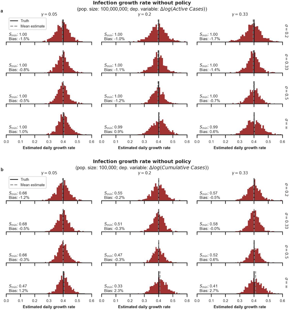
References


