
Abstract
Background The average treatment effect of antidepressants in major depression was found to be about 2 points on the 17-item Hamilton Depression Rating Scale, which lies below clinical relevance. Here, we searched for evidence of a relevant treatment effect heterogeneity that could justify the usage of antidepressants despite their low average treatment effect.
Methods Bayesian meta-analysis of 169 randomized, controlled trials including 58,687 patients. We considered the effect sizes log variability ratio (lnVR) and log coefficient of variation ratio (lnCVR) to analyze the difference in variability of active and placebo response. We used Bayesian random-effects meta-analyses (REMA) for lnVR and lnCVR and fitted a random-effects meta-regression (REMR) model to estimate the treatment effect variability between antidepressants and placebo.
Results The variability ratio was found to be very close to 1 in the best fitting models (REMR: 95% HPD = [0.98, 1.02], REMA: 95% HPD = [1.00, 1.02]), whereas the CVR REMA showed a reduced variability 95% HPD [0.80,0.84]. The Widely Applicable Information Criterion (WAIC) showed that the lnVR REMR and the lnVR REMA outperform the lnCVR REMA. The between-study variance τ2 under the REMA was found to be low (95% HPD [0.00, 0.00]).
Conclusions The published data from RCTs on antidepressants for the treatment of major depression is compatible with a near-constant treatment effect. Although it is impossible to rule out a substantial treatment effect heterogeneity, its existence seems rather unlikely. Since the average treatment effect of antidepressants falls short of clinical relevance, the current prescribing practice should be re-evaluated.
Introduction
Depression is one of the most frequent psychiatric disorders and poses a major burden for individuals and society; it affects more than 300 million people worldwide and is ranked as the single largest contributor to disability [1]. The first-line treatment usually consists of psychotherapy and/or pharmacotherapy with antidepressant drugs [2, 3]. Within the last decades, the number of prescriptions of antidepressants has continuously increased in several regions of the world [4, 5]. However, whether antidepressants are effective in the treatment of major depression has been a highly controversial debate for many years [6-9]. A recent meta-analysis by Cipriani et al. comprising 522 randomized, controlled trials (RCTs) of 21 antidepressants in 116□477 participants reported that all antidepressants were more effective than placebo in reducing depressive symptoms [10]. Based on these findings, a spokesman for the Royal College of Psychiatrists in the U.K. said that “the research would finally put to bed the controversy about antidepressants, as it clearly showed that these drugs work in lifting mood and helping most people with depression” [11]. In contrast, the authors of a recent re-analysis criticised this meta-analysis for not taking into account several biases, such as publication bias [12]. They concluded that “the evidence does not support definitive conclusions regarding the efficacy of antidepressants for depression in adults, including whether they are more efficacious than placebo for depression”.
Albeit these contradictory conclusions, both analyses used the same dataset.The so-called average treatment effect, which measures the difference in mean outcomes between active and control group, was about 2 points on the 17-item Hamilton Depression Rating Scale (HAMD-17) [13] in this dataset [12]. According to Leucht et al. [14], a reduction of up to 3 points on the HAMD corresponds to “no change” in the Clinical Global Impressions - Improvement Scale (CGI-I) [15] and the assumed threshold of clinical significance is 7 points [16]. Thus, a reduction of 2 points on the HAMD is not detectable by the treating physician and is presumably clinically irrelevant.
Crucially, Munkholm et al. [12] reported the average treatment effect as an outcome parameter, whereas Cipriani et al. [10] reported the odds ratio (OR) of “response rates”, signifying the fraction of patients crossing the rather arbitrary threshold of 50% in symptom reduction (“responders”). This approach translates into a number-needed-to-treat (NNT) of around 8-10 for “response” [17].
Consequently, the question of whether a categorisation of patients into so-called “responders” and “non-responders” is legitimate fundamentally determines whether antidepressants should be considered effective or ineffective in clinical practice. Since millions of people are prescribed these drugs, frequently for many years, the question of whether this categorisation is legitimate is of highest importance.
Categorisation of continuous variables
Categorising patients into “responders” and “non-responders” based on crossing an arbitrary threshold on a continuous scale has frequently been criticised by statisticians as it may lead to an artificial inflation of the measured treatment effect and to a loss of power [18, 19]. It may create the illusion of a subgroup of patients that benefit particularly well from a given treatment. However, a NNT of 8 is compatible with every patient having the exact same treatment effect of 2 points on the HAMD [12, 20]. Only if a substantial so-called treatment effect heterogeneity exists, meaning that there are true “responders” and “non-responders”, the calculation of response rates may be legitimate and the average treatment effect may not be an appropriate outcome measure. However, in the absence of clear evidence for a relevant treatment effect heterogeneity, the average treatment effect is the best predictor of the causal treatment effect [20, 21].
Treatment effect heterogeneity
Treatment effect heterogeneity describes the extent to which a treatment might affect different individuals differentially. In other words, some patients may benefit a lot, others may be harmed by a given treatment, possibly resulting in a null finding when only considering the average treatment effect in clinical trials. However, the existence of a clinically relevant treatment effect heterogeneity, albeit widely believed and intuitively plausible, has not been shown yet.
Investigation of treatment effect heterogeneity
Simply labeling patients as “responders” and “non-responders” based on crossing an arbitrary threshold on a continuous outcome scale is not a valid way to investigate variation in individual treatment effect [22]. In order to assess treatment effect heterogeneity from the data of parallel group trials, the comparison of variances between the active and the control condition has been proposed [22, 23]. Here, an increase in variance in the active group might be a signal of a variation in the individual treatment effect [22].
Following a recent publication by Winkelbeiner et al. [21], analyzing differences in variances in 52 randomized, placebo-controlled antipsychotic drug trials, the present analysis aimed to assess the evidence for individual antidepressant drug response using the open dataset of the largest meta-analysis of the efficacy of antidepressants in major depressive disorder [10]. Here, we addressed the following research question: What is the evidence for a relevant treatment effect heterogeneity of antidepressants in the treatment of depression that justifies their usage despite the lack of a clinically relevant average treatment effect?
Methods
Data Acquisition
We obtained the dataset of the meta-analysis by Cipriani et al. [10] from the Mendeley database (https://data.mendeley.com/datasets/83rthbp8ys/2). This study included all RCTs comparing 21 antidepressants with placebo or another active antidepressant as oral monotherapy for the acute treatment of adults (≥18 years old and of both sexes) with a primary diagnosis of major depressive disorder according to standard operationalized diagnostic criteria (Feighner criteria, Research Diagnostic Criteria, DSM-III, DSM-III-R, DSM-IV, DSM-5, and ICD-10). For further details on the inclusion criteria and study characteristics, see the original study [10].
Data extraction and processing
Of the total of 522 studies we kept the 304 that included a placebo arm. We excluded all studies for which the reported endpoint did not represent the change from baseline, leaving us with a total of 169 studies for the analysis (see PRISMA flow diagram, supplementary data, figure 1). We extracted both the mean and the standard deviation of pre- and post-treatment outcome difference scores (the “response”). The studies included in the data set comprised 8 different depression scales, namely HAMD-17, HAMD-21, HAMD-24, HAMD unspecified, HAMD-29, HAMD-31, Montgomery–Åsberg Depression Rating Scale (MADRS) and IDS-IVR-30 [25, 26]. Studies with different treatment arms were aggregated according to the recommendation of the Cochrane Collaboration [27]. In this manuscript, we define response as pre-post-difference of a given outcome scale.

Visualization of a hypothetical patient in a randomized placebo-controlled trial. The patient is randomized to either the placebo or the active arm, corresponding to two hypothetical “potential outcomes”. Only one of which can ever be observed, as a single patient cannot receive both placebo and the active intervention at the same time. The difference between the two potential outcomes corresponds to the “individual treatment effect” of the intervention (here, a clinically relevant difference of 10 HAMD-17 points). The individual treatment effect is unobservable and can be imaged to be drawn from hypothetical distributions of the treatment effect. The variance of this distribution corresponds to the treatment effect heterogeneity. The factor ρ is the correlation between the placebo response and the individual treatment effect. Here, we assume that a given patient has a fixed individual treatment effect.
Statistical Analysis
We considered two different effect size statistics as suggested by Nakagawa et al. [28] to analyze the difference in variability of active and placebo response.
The log variability ratio

The log coefficient of variation ratio

These two effect sizes differ in the way they account for differences in mean between the active and the placebo group. Whereas lnVR assumes no correlation between concurrent changes in mean response and standard deviation of response, lnCVR measures differences in variability between groups after accounting for differences in mean response. If the active and placebo arms have equal variance, a VR (or CVR) of 1 would be expected. A value greater than 1 indicates a larger variability in the active group.
A variability ratio that substantially differs from 1 implies a considerable treatment effect heterogeneity. Conversely, a VR of around 1 is compatible with a near-constant treatment effect, but does not exclude the existence of a treatment effect heterogeneity. It should be noted, that it is impossible to disprove the existence of a subgroup with a substantially greater than average effect. However, the magnitude of the treatment effect heterogeneity can be bounded by the distance of the variability ratio VR from the value 1.
All statistical analyses were carried out in the programming language Python (version 3.7) and the probabilistic programming language Stan (with pystan version 2.18.1.0 as a Python interface). We used a Bayesian approach to fit all our models using weakly informative priors. Firstly, we used a Bayesian random-effects meta-analyses (REMA) for the two effect statistics lnVR and lnCVR. Secondly, we used a Bayesian random-effects meta-regression (REMR) to fit the lnVR effect statistic with the natural logarithm of the response ratio (lnRR) as a regressor [28], which is defined as:
3. The log of the response ratio

An additional complexity in our analysis, as compared to recent analyses [21, 28-30], came from the fact that our data set contained several different depression scales (several versions of the HAMD and the MADRS, see supplementary figure 2). For our analysis we made the assumption that these different scales are (locally) linearly transformable into each other. This assumption is well supported by the literature [31]. Fortunately, the lnVR and lnCVR effect statistics are invariant under linear transformations of the outcome scale.

Linear association between lnMean and lnSD using a varying intercept model, where the intercepts are allowed to vary between studies with different depression scales. Red dots represent active groups, blue dots represent placebo groups.

Posterior credible intervals for the exp(µ) parameter for the different models. REMA: random-effects meta-analysis. FEMA: fixed-effects meta-analysis. REMR: random-effects meta-regression. Note that the results are very similar for the REMR and the lnVR meta-analyses.
Random-effects meta-analysis (REMA)
We applied a Bayesian random-effects meta-analysis in order to estimate the effect sizes ES=lnVR, lnCVR. For the REMA, the following model was applied, where µ equals the “true” mean of the effect size. Finally, η represents the between-study-variance.
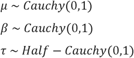
We specified the following weakly-informative hyper-priors:
Random-effects meta-regression (REMR)
This approach is a “contrast-based” version of the “arm-based” meta-analysis in Nakagawa et al. [28] which models the log of the standard deviation of the outcome directly in a multi-level meta-regression. For the REMR, the following model was applied, where µ equals the “true” mean of lnVR over all studies and X the “true” value of lnRR, if we account for measurement error. The variable β is the regression coefficient for X and thus signifies the degree of linear association between lnVR and lnRR. Finally, η represents the between-study-variance.
We specified the following weakly-informative hyper-priors:
Results
Study selection
As mentioned above, we included 169 placebo-controlled studies that reported mean and standard deviation of change in depression scores. These studies included data on 58,687 patients treated with 21 different antidepressants.
Correlation between mean and standard deviation of depression scores
In order to identify the more appropriate effect size (VR or CVR), we investigated the linear association between the mean response scores and their standard deviation using a varying intercept model, where the intercepts were allowed to vary between studies with different depression scales. Fitting a Bayesian varying intercept regression model with measurement error with lnMean as independent variable and lnSD as dependent variable, we get a posterior mean for the slope coefficient of 0.08 with a 95% HPD (highest probability density) interval of [0.03, 0.14]. This can be interpreted as a weak correlation between lnMean and lnSD of the order of +0.1. We remark that simply computing the correlation of the two quantities without paying attention to the correct weighting and the different scales in the data would yield an overestimated correlation of 0.41.
Log variability ratio (lnVR) and log coefficient of variation (lnCVR) models
In order to estimate the difference in variability between antidepressant and placebo response, we modelled the lnVR effect size using a Bayesian random effects model as heterogeneity between studies may be expected. The posterior mean estimate for the variability ratio was 1.01, with the 95 % highest posterior density (HPD) interval reaching from 1.00 to 1.02. The lnVR effect size assumes no correlation between lnMean and lnSD and may give biased results if such a correlation exists. In the presence of a positive correlation between mean and standard deviation, Nakagawa et al. [28] suggest that the lnCVR may be the more appropriate effect size to investigate the difference in variability between the active and control. The lnCVR REMA showed a reduction in the coefficient of variation in the active versus the placebo group (posterior mean estimate for CVR: 0.82, 95% HPD [0.80,0.84]).
Between-study heterogeneity
The between-study variance τ2 under the REMA was found to be low for both lnVR (95% HPD [0.00,0.00]) and lnCVR (95% HPD of τ2 [0.00,0.01]). Indeed, applying a fixed effects model instead of the REMA for the purpose of sensitivity analysis yielded similar results for the overall mean estimates of lnVR and lnCVR.
Random-effects meta-regression
Finally, we used a Bayesian random effects meta-regression (REMR). The advantage of this model over the lnVR and lnCVR meta-analyses is that we are not forced to make rigid assumptions about the association between the lnMean and lnSD, as the strength of this relationship is estimated directly from the data. Fitting this model, we obtained posterior statistics for the μ and β coefficients. The posterior mean estimate for eμ was 1.00 (95% HPD [0.98,1.02]) and that for β 0.04 (95% HPD [-0.03,0.12]), where we can (roughly, up to measurement error and random noise) interpret the coefficients as follows:
4.

Note that the lnVR REMA corresponds to a lnVR REMR with a β coefficient set to 0, whereas the lnCVR REMA corresponds to a lnVR REMR with a β coefficient set to 1. The REMR model learns the β coefficient and its posterior HDP interval is equal to 0.04 [-0.03, 0.12] suggesting that the lnVR REMA is a more appropriate model than the lnCVR REMA.
Performance comparison of the different models
In order to compare the performance of the different models applied, we used the so-called widely applicable information criterion (WAIC). This method estimates the pointwise prediction accuracy of fitted Bayesian models. Here, higher values of WAIC indicate a better out-of-sample predictive fit (“better” model). We refer to Vehtari et al. [32] for more details on WAIC. Figure 4 shows the logWAIC for the different models.

Widely applicable information criterion (WAIC) depicted on a logarithmic scale. Higher values signify a better predictive fit of the underlying model. Bars indicate standard errors. REMA: random-effects meta-analysis. FEMA: fixed-effects meta-analysis. REMR: random-effects meta-regression.
We observed that the lnVR REMA and the lnVR REMR outperformed the lnCVR REMA with respect to the WAIC. The difference between the lnVR REMA and the lnVR REMR showed comparable performance with respect to the WAIC.
Discussion
The efficacy of antidepressants in the treatment of major depressive disorder has been the topic of an ongoing debate for years in the psychiatric community and the public [6-9]. In a recent re-analysis [12] of a network meta-analysis [10], the average treatment effect of antidepressants was found to be about 2 points on the HAMD-17 scale, which is almost undetectable by clinicians [14] and clearly lies below the assumed minimally clinically relevant effect of 7 points [16]. In addition, it should be noted that relevant biases may have led to an overestimation of the drugs’ efficacy [12, 33]. Jakobsen et al. recently concluded that, based on current evidence, antidepressants should not be used in adult patients with major depressive disorder [34].
Evidence for treatment effect heterogeneity
On the basis of these facts, the question arises as to why these compounds are considered to be effective nevertheless. The main reason for this might be the assumption of a substantial treatment effect heterogeneity, meaning that subpopulations of patients exist that benefit substantially more than average from the medication. If the treatment effect heterogeneity is low, no patient would have a clinically relevant benefit. In the face of the well documented harms and side effects, antidepressants may then not be considered useful in the treatment of major depression. We believe that the use of antidepressants may only be justified, if the treatment effect heterogeneity is sufficiently large, such that at least some patients have a clinically relevant benefit.
Albeit widely believed and putatively observed in clinical routine, substantial differences in the individual treatment effect of antidepressants have not been shown to exist yet. A “responder”, usually defined as someone crossing an arbitrary threshold of symptom severity, is a person who was observed to improve and not necessarily caused by the medication to get better. Even constant treatment effects lead to differences in observed response rates, creating the illusion of a differential treatment effect, where none exists [20]. Therefore, the frequently performed calculation of response rates is misleading and seems inappropriate to answer the question of treatment effect heterogeneity.
This work aimed to estimate the treatment effect heterogeneity of antidepressants in the treatment of major depressive disorder using a large dataset of a recent network meta-analysis [10]. To this end, we applied the effect size statistics lnVR and lnCVR suggested by Nakagawa et al. [28], using a Bayesian random-effects meta-analytical approach (REMA) and fitted a multi-level meta-regression (REMR) model to estimate the treatment effect variability between antidepressants and placebo. Both the lnVR REMR and the lnVR REMA, which were found to outperform the lnCVR REMA, showed that the variability ratio was very close to 1 (REMR: 95% HPD = 0.98 to 1.02, REMA: 95% HPD = 1.00 to 1.02), perfectly compatible with a near-constant effect of antidepressants on depression severity in all patients. These findings are in line with those of a recently published meta-analysis of antidepressants using the same dataset [35].
Methodological aspects
In order to determine the variability of the treatment response, the correlation between the mean and standard deviation of the underlying measuring scale has to be taken into account. The lnVR and the lnCVR effect sizes naively assume a slope coefficient of 0 and 1, respectively. In other words, how much of the (logarithmic) difference in variances is explained by the difference in (logarithmic) means. Both scales may thus give biased results, if the true slope coefficient is near 0.5.
Our work adds accuracy to the existing literature, as we developed a generalized model (REMR) that incorporates the correlation between mean and standard deviation directly from the data. Applying this model yielded a mean estimate for the VR of 1.00 (95% HPD [0.98,1.02]).
By applying a varying intercept model, taking into account the occurrence of different depression scales, we could show that the correlation between (logarithmic) mean and (logarithmic) standard deviation is of a very small magnitude (slope coefficient = 0.08), indicating that the lnVR is a more appropriate measure as opposed to the lnCVR. A regression over all depression scales yields a correlation coefficient of 0.4, which is 5 x as large as our estimate. When simply conducting a significance test for the existence of such correlation, the lnCVR effect size would appear to be the appropriate measure, leading to the incorrect conclusion of a substantially reduced variability in the active arm. It is important to note that a VR (or CVR) sufficiently smaller than 1 is in fact evidence of treatment effect heterogeneity. Therefore, considering the lnCVR as the main outcome would lead to the opposite conclusion of substantial treatment effect heterogeneity [30].
We applied the WAIC in order to estimate the predictive power of our models. This effect measure showed the REMR model and the lnVR effect size had better out of sample predictive power than the lnCVR.
How should these results inform clinical practice?
The VR is a measure that can potentially detect evidence for subgroups that benefit (substantially) more than average from an intervention. A VR that differs substantially from 1 is evidence of such subgroups (of large treatment effect heterogeneity), while a VR near 1 is compatible with both a small and a large treatment effect heterogeneity. A VR of exactly 1 (which is the mean-estimate of our REMR model) would be proof of a constant treatment effect. It is, however, impossible to ever prove identity, as we can never reach an uncertainty of 0 (credible interval with width of 0). Furthermore, an exactly constant treatment effect seems impossible also from a theoretical point of view. So how should a VR of 1 (95% HPD [0.98,1.02]) be interpreted? For this, consider the following illustration:
Hypothesis 1 (H1): The treatment effect heterogeneity is close to 0 (e.g. 99% of patients have an individual treatment effect of 1 to 3 HAMD points).
Hypothesis 2 (H2): The treatment effect heterogeneity is greater than in H1.
There are now three possibilities:
H1 is true and VR ∼ 1 (very close to 1, e.g. 0.98 to 1.02)
H2 is true and VR ∼ 1
H2 is true and VR ≠ 1 (not very close to 1)
Our results indicate that VR ∼ 1. We can thus rule out one of the three possibilities, namely a large treatment heterogeneity combined with a VR ≠ 1. From a Bayesian perspective, the probability of H1 being true increases, while that of H2 being true decreases. How we now regard the probability of H1 or H2 being true depends on how plausible we considered these scenarios to begin with (the prior probabilities).
In order for H2 to be true and the VR being close to 1, a strong correlation between the placebo response and the treatment effect of antidepressants would be necessary. Since no benefitting subpopulations have been identified to date, such a correlation seems unlikely. If those patients whose depression severity would remain unchanged under placebo would have the strongest antidepressant medication effect, we might expect patients with certain features (such as chronic depression) to benefit substantially more than average from antidepressants. This has not been shown to be the case.
Conclusion
This work could show that the published data from RCTs on antidepressant medication in major depression is compatible with a near-constant treatment effect, which is also the simplest explanation for the observed data. Although it is not possible to rule out a substantial treatment effect heterogeneity using summary data from RCTs, a substantial treatment effect heterogeneity seems unlikely. Until the existence of benefiting subgroups has been demonstrated prospectively, the average treatment effect is the best estimator of the individual treatment effect. Since the average treatment effect of antidepressants probably falls short of clinical relevance, the current prescribing practice in the treatment of major depression should be critically re-evaluated.
Python code
Statement of Ethics
The authors have no ethical conflicts to disclose.
Data Availability
The raw data is available online. We will upload the python code with all performed analyses.
Disclosure Statement
CAM received consulting fees from Silence Therapeutics, outside the submitted work. The other authors declared no competing interest. All authors declare no other relationships or activities that could appear to have influenced the submitted work. No funder had any role in: the design and conduct of the study; collection, management, analysis, and interpretation of the data; preparation, review, or approval of the manuscript; and decision to submit the manuscript for publication.
Funding Sources
The authors received no specific funding for this work.
Author Contributions
Study idea and design: CV and CAM. Data extraction, statistical analyses: AV and CV. Mathematical modelling and code implementation: AV. All authors contributed to drafting the manuscript. All authors provided a critical review and approved the final paper.
References


