
Abstract
Since the first suspected case of novel coronavirus (2019-nCoV)–infected pneumonia (NCIP) on December 1st, 2019, in Wuhan, Hubei Province, China, a total of 40,235 confirmed cases and 909 deaths have been reported in China up to February 10, 2020, evoking fear locally and internationally. Here, based on the publicly available epidemiological data (WHO, CDC, ECDC, NHC and DXY) for Hubei from January 11 to February 10, 2020, we provide estimates of the main epidemiological parameters, i.e. the basic reproduction number (R0) and the infection, recovery and mortality rates, along with their 90% confidence intervals. As the number of infected individuals, especially of those with asymptomatic or mild courses, is suspected to be much higher than the official numbers, we have repeated the calculations under a scenario that considers five times the number of confirmed infected cases and eight times the number of recovered. Our computations and analysis were based on a mean field Susceptible-Infected-Recovered-Dead (SIRD) model. Thus, based on the SIRD simulations, the estimated average value of R0 was found to be 2.5, while the one computed by the official counts of the confirmed cases from the 11th of January until the 18th of January was found to be 4.6. Furthermore, on the estimated parameters from both scenarios, we provide tentative three-week forecasts of the evolution of the outbreak at the epicenter. Our forecasting flashes a note of caution for the presently unfolding outbreak in China. Based on the official counts for confirmed cases, the cumulative number of infected will surpass 68,000 (as a lower bound) and could reach 140,000 (with an upper bound of 290,000) by February 29. Regarding the number of deaths, simulations forecast that on the basis of current data and estimations on the official count of infected people in the population, the death toll might exceed 7,000 by February 29; however, our analysis further reveals a significant decline of the mortality rate to which various factors may have contributed, such as the severe control measures taken in Hubei, China (e.g. quarantine and hospitalization of infected individuals), but also a high underestimation of the number of infected and recovered people in the population, which will hopefully lower the death toll.
1 Introduction
An outbreak of “pneumonia of unknown etiology” in Wuhan, Hubei Province, China in early December 2019 has spiraled into an epidemic that is ravaging China and threatening to reach a pandemic state [1]. The causative agent soon proved to be a new betacoronavirus related to the Middle East Respiratory Syndrome virus (MERS-CoV) and the Severe Acute Respiratory Syndrome virus (SARS-CoV). The novel coronavirus has been tentatively named “2019-nCoV” by the World Health Organization (WHO) and on January 30, the 2019-nCoV outbreak was declared to constitute a Public Health Emergency of International Concern by the WHO Director-General [2]. Despite the lockdown of Wuhan and the suspension of all public transport, flights and trains on January 23, a total of 40,235 confirmed cases, including 6,484 (16.1%) with severe illness, and 909 deaths (2.2%) had been reported in China by the National Health Commission up to February 10, 2020; meanwhile, 319 cases and one death were reported outside of China, in 24 countries [3]. The origin of 2019-nCoV has not yet been determined although preliminary investigations are suggestive of a zoonotic, possibly of bat, origin [4, 5]. Similarly to SARS-CoV and MERS-CoV, the novel virus is transmitted from person to person principally by respiratory droplets, causing such symptoms as fever, cough, and shortness of breath after a period believed to range from 2 to 14 days following infection, according to the Centers for Disease Control and Prevention (CDC) [1, 6, 7]. Preliminary data suggest that older males with comorbidities may be at higher risk for severe illness from 2019-nCoV [6, 8, 9]. However, the precise virologic and epidemiologic characteristics, including transmissibility and mortality, of this third zoonotic human coronavirus are still unknown. Using the serial intervals (SI) of the two other well-known coronavirus diseases, MERS and SARS, as approximations for the true unknown SI, Zhao et al. estimated the mean basic reproduction number (R0) of 2019-nCoV to range between 2.24 (95% CI: 1.96-2.55) and 3.58 (95% CI: 2.89-4.39) in the early phase of the outbreak [10]. Very similar estimates, 2.2 (95% CI: 1.4-3.9), were obtained for R0 at the early stages of the epidemic by Imai et al. 2.6 (95% CI: 1.5-3.5) [11], as well as by Li et al., who also reported a doubling in size every 7.4 days [1]. Wu et al. estimated the R0 at 2.68 (95% CI: 2.47–2.86) with a doubling time every 6.4 days (95% CI: 5.8–7.1) and the epidemic growing exponentially in multiple major Chinese cities with a lag time behind the Wuhan outbreak of about 1–2 weeks [12]. Amidst such an important ongoing public health crisis that also has severe economic repercussions, we reverted to mathematical modelling that can shed light to essential epidemiologic parameters that determine the fate of the epidemic [13]. Here, we present the results of the analysis of time series of epidemiological data available in the public domain (WHO, CDC, ECDC, NHC and DXY) from January 11 to February 10, 2020, and attempt a three-week forecast of the spreading dynamics of the emerged coronavirus epidemic in the epicenter in mainland China.
2 Methodology
Our analysis was based on the publicly available data of the new confirmed daily cases reported for the Hubei province from the 11th of January until the 10th of February. Based on the released data, we attempted to estimate the mean values of the main epidemiological parameters, i.e. the basic reproduction number R0, the infection (α), recovery (β) and mortality rate (γ), along with their 90% confidence intervals. However, as it has been suggested [14], the number of infected, and consequently the number of recovered, people is likely to be much higher. Thus, in a second scenario, we have also derived results by taking five times the number of reported cases for the infected and recovered cases, while keeping constant the number of deaths that is more likely to be closer to the real number. Based on these estimates we also provide tentative forecasts until the 29th of February. Our methodology follows a two-stage approach as described below.
The basic reproduction number is one of the key values that can predict whether the infectious disease will spread into a population or die out. R0 represents the average number of secondary cases that result from the introduction of a single infectious case in a totally susceptible population during the infectiousness period. Based on the reported data of confirmed cases, we provide estimations of the R0 from the 16th up to the 20th of January in order to satisfy as much as possible the hypothesis of S = N that is a necessary condition for the computation of R0. We also provide estimations of β, γ over the entire period using a rolling window of one day from the 11th of January to the 16th of January to provide the very first estimations.
Furthermore, we exploited the SIRD model to provide an estimation of the infection rate α. This is accomplished by starting with one infected person on the 16th of November, which has been suggested as a starting date of the epidemic [6], run the SIR model until the 10th of February and optimize α to fit the reported confirmed cases from the 11th of January to the 10th of February. Below, we describe analytically our approach. Let us start by denoting with S(t), I(t), R(t), D(t), the number of susceptible, infected, recovered and dead persons respectively at time t in the population of size N. For our analysis we assume that the total number of the population remains constant. Based on the demographic data for the province of Hubei N = 59m. Thus, the discrete SIRD model reads:


Initially, when the spread of the epidemic starts, all the population is considered to be susceptible, i.e. S ≈ N. Based on this assumption, by Eq.(2),(3),(4), the basic reproduction number can be estimated by the parameters of the SIRD model as:

A problem with the approximation of the epidemiological parameters α, β and γ and thus R0, from real-world data based on the above expressions is that in general, for large scale epidemics, the actual number of infected I(t) persons in the whole population is unknown. Thus, the problem is characterized by high uncertainty. However, one can attempt to provide some coarse estimations of the epidemiological parameters based on the reported confirmed cases using the approach described next.
2.1 Identification of epidemiological parameters from the reported data of confirmed cases
Lets us denote with ΔI(t), ΔR(t), ΔD(t), the reported new cases of infected, recovered and deaths at time t, with CΔI(t), CΔR(t), CΔD(t) the cumulative numbers of confirmed cases at time t. Thus:
 where, X = I, R, D.
Let us also denote by CX(t) = [CX(1), CX(2), …, CX(t)]T, the t×1 column vector containing the corresponding cumulative numbers up to time t. On the basis of Eqs.(2), (4), one can provide a coarse estimation of the parameters R0, β and γ as follows.
Starting with the estimation of R0, we note that as the province of Hubei has a population of 59m, one can reasonably assume that for any practical means, at least at the beginning of the outbreak, S ≈ N. By making this assumption, one can then provide an approximation of the expected value of R0 using Eq.(5) and Eq.(2), Eq.(3), Eq.(4). In particular, substituting in Eq.(2), the terms βI(t − 1) and γI(t − 1) with ΔR(t) = R(t) − R(t − 1) from Eq.(3), and ΔD(t) = D(t) − D(t − 1) from Eq.(4) and bringing them into the left-hand side of Eq.(2), we get:

Adding Eq.(3) and Eq.(4), we get:

Finally, assuming that for any practical means at the beginning of the spread that S = N and dividing Eq.(7) by Eq.(8) we get:

Thus, based on the above, a coarse estimation of R0 and its corresponding confidence intervals can be provided by solving a linear regression problem using least-squares problem as:

For the estimation of the recovery and mortality rates, we adopt the formula that uses the National Health Commission (NHC) of the People’s Republic of China [15], that is the ratio of the cumulative number of recovered/deaths and that of infected at time t. Thus, a coarse estimation of the mortality rate γ (and in a similar way of the recovery rate) can be calculated solving a linear regression problem by least squares as:

Here, we have repeated the above calculations by taking five times the reported number of infected and eight times the reported number of recovered in the population, while leaving the reported number of deaths the same.
2.2 Estimation of the infection rate from the SIRD model
Having estimated the expected values of the parameters β and γ, an approximation of the infected rate α, that is not biased by the assumption of S = N can be obtained by using the SIRD simulator. In particular, in the SIRD model we set  and
and  , and set as initial conditions one infected person on the 16th of November and run the simulator until the last date for which there are available data (here up to the 10th of February). Then, the value of the infection rate α can be found by “wrapping” around the SIRD simulator an optimization algorithm (such as a nonlinear least-squares solver) to solve the problem:
 where
where
 where,
  are the differences between the cumulative new cases of the infected, recovered and dead people resulting from the SIRD simulator and the reported (or, in the second scenario the five times the reported infected and recovered) real-world cumulative cases at time t; w1, w2, w3 correspond to scalars serving in the general case as weights to the relevant functions. For the solution of the above optimization problem use used the function “lsqnonlin” of matlab [16] using the Levenberg-Marquard algorithm.
3 Results
As discussed, we have derived results using two different scenarios (see in Methodology). For each scenario, we first present the results obtained by solving the least squares problem as described in section 2.1 using a rolling window of an one-day step. The first time window was that from the 11th up to the 16th of January i.e. we used the first six days to provide the very first estimations of the epidemiological parameters. We then proceeded with the calculations by adding one day in the rolling window as described in the methodology. For each window, we also report, the corresponding coefficients of determination (R2) representing the proportion of the variance in the dependent variable that is predictable from the independent variables, and the root mean square of error (RMSE). Then, we used the SIRD model to provide an estimation of infection rate by “wrapping” around the SIRD simulator the optimization algorithm as described in section 2.2. Finally, we provide tentative forecasts for the evolution of the outbreak based on both scenarios until the end of February.
3.1 Scenario I: Results obtained using the exact numbers of the reported confirmed cases
Figure1 depicts an estimation of R0 for the period January 16-January 20. Using the first six days from the 11th of January,  results in ∼ 4.80 (90% CI: 3.35-6.27); using the data until January 17,
  results in ∼ 4.60 (90% CI: 3.56-5.65); using the data until January 18,
  results in ∼ 5.14 (90%CI: 4.25-6.04); using the data until January 19,
  results in ∼ 6.09 (90% CI: 5.02-7.16); and using the data until January 20,
  results in ∼ 7.09 (90% CI: 5.84-8.35) Figure2 depicts the estimated values of the recovery (β) and mortality (γ) rates for the period January 16 to February until the 10th of February, the estimated value of the mortality rate γ is ∼2.94% (90% CI: 2.89%-3.0%) and that of the recovery rate is ∼0.05 (90% CI: 0.045-0.055) corresponding to ∼20 days (90% CI: 18-22). However, it is interesting to note that as the available data become more, the estimated recovery rate increases significantly from the 31th of January (see Fig.2).

Scenario I. Estimated values of the basic reproduction number (R0) as computed by least squares using a rolling window with initial date the 11th of January. The solid line corresponds to the mean value and dashed lines to lower and upper 90% confidence intervals

Scenario I. Estimated values of the recovery  and mortality
  rate as computed by least squares using a rolling window (see section 2.1). Solid lines correspond to the mean values and dashed lines to lower and upper 90% confidence intervals
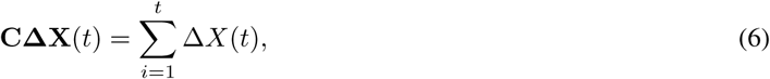
In Figures 3,4,5, we show the coefficients of determination (R2) and the root of mean squared errors (RMSE), for  and
and  , respectively.

Scenario I. Coefficient of determination (R2) and root mean square error (RMSE) resulting from the solution of the linear regression problem with least-squares for the basic reproduction number (R0)
Scenario I. Coefficient of determination (R2) and root mean square error (RMSE) resulting from the solution of the linear regression problem with least-squares for the recovery rate (β)

Scenario I. Coefficient of determination (R2) and root mean square error (RMSE) resulting from the solution of the linear regression problem with least-squares for the mortality rate (γ)
As described in the methodology, we have also used the SIRD simulator to provide an estimation of the infection rate by optimization with w1=1, w2=2, w3=2. Thus, we performed the simulations by setting β=0.05 and γ=0.0294, and as initial conditions one infected, zero recovered and zero deaths on November 16th 2019, and run until the 10th of February. The optimal, with respect to the reported confirmed cases from the 11th of January to the 10th of February, value of the infected rate (α) was ∼0.199 (90% CI: 0.197-0.201). This corresponds to a mean value of the basic reproduction number  . Note that this value is different compared to the value that was estimated using solely the reported data.
Finally, using the derived values of the parameters α, β, γ, we have run the SIRD simulator until the end of February. The results of the simulations are given in Figures6,7,8. Solid lines depict the evolution, when using the expected (mean) estimations and dashed lines illustrate the corresponding lower and upper bounds as computed at the limits of the confidence intervals of the estimated parameters.

Scenario I. Simulations until the 29th of February of the cumulative number of infected as obtained using the SIRD model. Dots correspond to the number of confirmed cases from the 16th of January to the 10th of February. The initial date of the simulations was the 16th of November with one infected, zero recovered and zero deaths. Solid lines correspond to the dynamics obtained using the estimated expected values of the epidemiological parameters α = 0.199, β = 0.05, γ = 0.0294

Scenario I. Simulations until the 29th of February of the cumulative number of recovered as obtained using the SIRD model. Dots correspond to the number of confirmed cases from the 16th of January to the 10th of February. The initial date of the simulations was the 16th of November with one infected, zero recovered and zero deaths. Solid lines correspond to the dynamics obtained using the estimated expected values of the epidemiological parameters α = 0.199, β = 0.05, γ = 0.0294

Scenario I. Simulations until the 29th of February of the cumulative number of deaths as obtained using the SIRD model. Dots correspond to the number of confirmed cases from 16th of January to the 10th of February. The initial date of the simulations was the 16th of November with one infected, zero recovered and zero deaths. Solid lines correspond to the dynamics obtained using the estimated expected values of the epidemiological parameters α = 0.199, β = 0.05, γ = 0.0294
As Figures 6,7 suggest, the forecast of the outbreak at the end of February, through the SIRD model is characterized by a high uncertainty. In particular, simulations result to an expected number of ∼140,000 infected cases but with a high variation: the lower bound is at ∼70,000 infected cases while the upper bound is at ∼290,000 cases. Similarly for the recovered population, simulations result to an expected number of ∼60,000, while the lower and upper bounds are at ∼33,000 and ∼95,000, respectively. Finally, regarding the deaths, simulations result to an average number of ∼16,000, with lower and upper bounds, ∼9000 and ∼29,000, respectively. However, as more data are released it appears that the mortality rate is lower than the predicted with the current data and thus the death toll is expected, hopefully to be significantly less compared with then predictions.
3.3 Scenario II. Results obtained based by taking five times the number of infected and eight times the number of recovered people with respect to the confirmed cases
For our illustrations, we assumed that the number of infected is five times the number of the confirmed infected and eight times the number of the confirmed recovered people. Figure9 depicts an estimation of R0 for the period January 16-January 20. Using the first six days from the 11th of January to 16th of January,  results in 4.15 (90% CI: 2.92-5.38); using the data until January 17,
  results in 3.98 (90% CI: 3.11-4.85); using the data until January 18,
  results in 4.39 (90% CI: 3.67-5.11); using the data until January 19,
  results in 5.15 (90% CI: 4.30-6.01) and using the data until January 20,
  results in 6.01 (90% CI: 4.93-7.08)

Scenario II. Estimated values of the basic reproduction number (R0) as computed by least squares using a rolling window with initial date the 11th of January. The solid line corresponds to the mean value and dashed lines to lower and upper 90% confidence intervals.
Figure10 depicts the estimated values of the recovery (β) and mortality (γ) rates for the period January 16 to February 10. The confidence intervals are also depicted with dashed lines. Using all the available data from the 11-th of January until the 10th of February, the estimated value of the mortality rate γ now drops to ∼0.58% (90% CI: 0.57%-0.59%) while that of the recovery rate is ∼0.08 (90% CI: 0.073-0.088) corresponding to ∼12 days (90% CI: 11-13). It is interesting also to note, that as the available data become more, the estimated recovery rate increases (see Fig.10), while the mortality rate seems to be stabilized in the rate of ∼ 0.58%.

Scenario II. Estimated values of the recovery  rate and mortality
  rate, as computed by least squares using a rolling window (see section 2.1). Solid lines correspond to the mean values and dashed lines to lower and upper 90% confidence intervals
In Figures 11,12,13, we show the coefficients of determination (R2) and the root of mean squared errors (RMSE), for  and
and  , respectively.

Scenario II. Coefficient of determination (R2) and root mean square error (RMSE) resulting from the solution of the linear regression problem with least-squares for the basic reproduction number (R0)

Scenario II. Coefficient of determination (R2) and root mean square error (RMSE) resulting from the solution of the linear regression problem with least-squares for the recovery rate (β)

Scenario II. Coefficient of determination (R2) and root mean square error (RMSE) resulting from the solution of the linear regression problem with least-squares for the mortality rate (γ)
Again, we used the SIRD simulator to provide estimation of the infection rate by optimization with with w1 = 1, w2 = 2, w3 = 2. Thus, to find the optimal infection run, we used the SIRD simulations with β = 0.08, and γ = 0.0058 and as initial conditions one infected, zero recovered, zero deaths on November 16th 2019, and run until the 10th of February. The optimal, with respect to the reported confirmed cases from the 11th of January to the 10th of February value of the infected rate (α) was ∼0.227 (90% CI: 0.224-0.229). This corresponds to a mean value of the basic reproduction number  . Finally, using the derived values of the parameters α, β, γ, we have run the SIRD simulator until the end of February. The simulation results are given in Figures14,15,16. Solid lines depict the evolution, when using the expected (mean) estimations and dashed lines illustrate the corresponding lower and upper bounds as computed at the limits of the confidence intervals of the estimated parameters.

Scenario II. Simulations until the 29th of February of the cumulative number of infected as obtained using the SIRD model. Dots correspond to the number of confirmed cases from 16th of Jan to the 10th of February. The initial date of the simulations was the 1st of Dec with one infected, zero recovered and zero deaths. Solid lines correspond to the dynamics obtained using the estimated expected values of the epidemiological parameters α = 0.227, β = 0.08, γ = 0.0058

Scenario II. Simulations until the 29th of February of the cumulative number of recovered as obtained using the SIRD model. Dots correspond to the number of confirmed cases from 16th of January to the 10th of February. The initial date of the simulations was the 16th of November, with one infected, zero recovered and zero deaths. Solid lines correspond to the dynamics obtained using the estimated expected values of the epidemiological parameters α = 0.227, β = 0.08, γ = 0.0058

Scenario II. Simulations until the 29th of February of the cumulative number of deaths as obtained using the SIRD model. Dots correspond to the number of confirmed cases from the 16th of November to the 10th of February. The initial date of the simulations was the 16th of November with zero infected, zero recovered and zero deaths. Solid lines correspond to the dynamics obtained using the estimated expected values of the epidemiological parametersα = 0.227, β = 0.08, γ = 0.0058
Again as Figures 15,16 suggest, the forecast of the outbreak at the end of February, through the SIRD model is characterized by a high uncertainty. In particular, in Scenario II, simulations result to an expected number of 1m infected cases in the whole population with a lower bound at 330,000 and an upper bound at ∼2.2m cases. Similarly, for the recovered population, simulations result to an expected number of 580,000, while the lower and upper bounds are at 230,000 and 960,000, respectively. Finally, regarding the deaths, simulations under this scenario result to an average number of 19,000, with lower and upper bounds, 7000 and 35,000.
Table 1 summarizes all the above results.
Model parameters, their computed values and forecasts for the Hubei province under two scenarios: (I) using the exact values of confirmed cases or (II) using estimations for infected and recovered (five and eight times the number of confirmed cases, respectively).
At this point we should make clear and underline that the above forecasts should not be considered by any means as actual/ real world predictions for the evolution of the epidemic as they are based on yet incomplete knowledge of the characteristics of the epidemic, the very high uncertainty regarding the actual number of already infected and recovered people and the effect of the measured already taken to combat the epidemic.
4 Discussion and Concluding Remarks
In the digital and globalized world of today, new data and information on the novel coronavirus and the evolution of the outbreak become available at an unprecedented pace. Still, crucial questions remain unanswered and accurate answers for predicting the dynamics of the outbreak simply cannot be obtained at this stage. We emphatically underline the uncertainty of available official data, particularly pertaining to the true baseline number of infected (cases), that may lead to ambiguous results and inaccurate forecasts by orders of magnitude, as also pointed out by other investigators [1, 14, 17]. Of note, 2019-nCoV, which is thought to be principally transmitted from person to person by respiratory droplets and fomites without excluding the possibility of the fecal-oral route [18] had been spreading for at least over a month and a half before the imposed lockdown and quarantine of Wuhan on January 23, having thus infected unknown numbers of people. The number of asymptomatic and mild cases with subclinical manifestations that probably did not present to hospitals for treatment may be substantial; these cases, which possibly represent the bulk of the 2019-nCoV infections, remain unrecognized, especially during the influenza season [17]. This highly likely gross under-detection and underreporting of mild or asymptomatic cases inevitably throws severe disease courses calculations and death rates out of context, distorting epidemiologic reality. Another important factor that should be taken into consideration pertains to the diagnostic criteria used to determine infection status and confirm cases. A positive PCR test was required to be considered a confirmed case by China’s Novel Coronavirus Pneumonia Diagnosis and Treatment program in the early phase of the outbreak [19]. However, the sensitivity of nucleic acid testing for this novel viral pathogen may only be 30-50%, thereby often resulting in false negatives, particularly early in the course of illness. To complicate matters further, the guidance changed in the recently-released fourth edition of the program on February 6 to allow for diagnosis based on clinical presentation, but only in Hubei province [19]. The swiftly growing epidemic seems to be overwhelming even for the highly efficient Chinese logistics that did manage to build two new hospitals in record time to treat infected patients. Supportive care with extracorporeal membrane oxygenation (ECMO) in intensive care units (ICUs) is critical for severe respiratory disease. Large-scale capacities for such level of medical care in Hubei province, or elsewhere in the world for that matter, amidst this public health emergency may prove particularly challenging. We hope that the results of our analysis contribute to the elucidation of critical aspects of this outbreak so as to contain the novel coronavirus as soon as possible and mitigate its effects regionally, in mainland China, and internationally.
Data Availability
All data referred to in the manuscript are available.
https://gisanddata.maps.arcgis.com/apps/opsdashboard/index.html#/bda7594740fd40299423467b48e9ecf6
Footnotes
lucia.russo{at}cnr.it
atsakris{at}med.uoa.gr
constantinos.siettos{at}unina.it


